Supplementary Materials
BNArray: An R package for constructing gene regulatory networks from microarray data by using Bayesian network
Authors: Xiaohui Chen, Ming Chen, Kaida Ning
Summary:
BNArray is a systemized tool developed in R. It facilitates the construction of gene regulatory networks from DNA microarray data by using Bayesian network. Significant submodules of regulatory networks with high confidence are reconstructed using our extended sub-network mining algorithm for directed graphs.
To evaluate the statistical features of generated Bayesian networks, re-sampling procedure are utilized to yield collection of candidates networks. These 1st-order network sets are used to mine dense coherent sub-networks. Additionally, BNArray can handle microarray data sets with missing data.
BNArray package is implemented in R, an open source programming environment. It has four main function modules:
1. Imputing missing data in microarray experiments with LLSimpute algorithm. Thus, we can input complete database for constructing Bayesian networks.
2. Constructing Bayesian networks for gene regulation. We utilize previously implemented R package deal for learning Bayesian networks with mixed variables.
3. Re-sampling microarray data set to produce more reliable data using Efron's Bootstrap, and then repeating procedure 2 to construct a collection of 1st-order Bayesian networks with high scores.
4. Reconstructing significant coherent regulatory sub-networks with our extended CODENSE algorithm for directed graph from previously induced candidate Bayesian networks.
BNArray allows users to specify their own parameters and modify the open source code to meet their individual needs.
Contents:
This document contains three parts:
Part I: Introduction to BNArray
Part II: Download & Utilization
Part I: Introduction to BNArray
The genome project has vastly increased our knowledge of the genomic sequences and their encoding products of human and many other model organisms. DNA microarray is one of the most powerful techniques developed to survey the transcriptional profile of the entire genome. It can measure the state of living cell in one experiment. Detailed laboratory protocols of microarray experiments have been developed in the past few years. Still the computational issues of the generated data remain arguable when dealing with specific situations.
Recently, Bayesian network, a probabilistic graphical model representation, has been widely used to analyze expression data. Compared with clustering analysis, Bayesian network has the advantage of uncovering conditional independency among genes, which provides a promising way to survey direct interaction of gene regulation. Moreover, by using statistical evaluation approaches, we can examine features of induced high score networks. For example, the confidence of the existence of an edge can be evaluated. Thus, high confident features provide us a potential way to mine significant sub-networks from candidate Bayesian networks. CODENSE, an efficient and fast algorithm for identifying coherent network modules from across multiple network collections, is used to reconstruct 2nd-order graphs from each undirected 1st-order network set.
So far, by using the Bayesian framework there is no tool to implement a systemized process for sub-regulatory networks for reconstruction from large scale DNA microarray data. We have developed an R package BNArray which provides a flexible interface for conducting this analysis. Furthermore, we extend the CODENSE algorithm to xCODENSE which mines coherent modules from a collection of directed graphs.
Input definition: BNArray reads microarray data from *.txt or plain text file delimited by Tab separators. Rows contain expression measures of one gene across various experiments and each column denotes the expression measured in one microarray slide (except the first column which is the names of genes). The following is an example of input format (using command df.all[1:5,1:6]):
| cln3-1 | cln3-2 | Clb2-2 | clb2-1 | Alpha |
YAL001C | 0.15 |
| -0.22 | 0.07 | -0.15 |
YAL002W | -0.07 | -0.76 | -0.12 | -0.25 | -0.11 |
YAL003W | -1.22 | -0.27 | -0.1 | 0.23 | -0.14 |
YAL004W | -0.09 | 1.2 | 0.16 | -0.14 | -0.02 |
We also attached a sample procedure to read the original .txt files into R type object df.ori, which contains the measurement data of differentially expressed genes from their names.
To initiate BNArray, we should first set the working directory to the one that contains the microarray files, and then load package deal to export functions for constructing general Bayesian networks. We use the demo wrapped in BNArray to illustrate the usage. Before conducting any analysis, data should be imported:
Note: we can optionally use
> attach(total.data)
In order to make each of later used data visible under their component names without need to quote total.data domain name, we attach total.data to the search path.
The current version of BNArray (V1.0) allows using Least Local Squares algorithm to estimate the missing values as the linear combination of their nearest neighbors:
> ori.compact <- LLSimpute(total.data$df.all, total.data$df.ori, total.data$n.changed)
Note: If we have attached total.data to search path, there is no need to addtotal.data$ before each component name.
LLSimpute function accepts data.frame objects df.all & df.ori with missing values from microarray expression data, and returns a matrix object with imputed values. Note that if a gene is missing too many values, LLSimpute cannot estimate a coefficient for these missing values. We call these values too bad data. Thus, for ensuring a complete database, we call function FinalImpute after LLSimpute:
> ori.compact <- FinalImpute(ori.compact)
FinalImpute procedure imputes too bad data to a specified value, e.g. zero, which means the expression levels cannot be detected in these experiments.
Finally, we cast ori.compact to the suitable R data type for Bayesian network construction procedure:
> bn.data <- PrepareCompData(ori.compact)
We implement Bayesian network learning by using deal package with a slight modification.
First, differentially expressed genes to be modeled are selected. For example, we select a subset of bn.data containing m=5 genes with n=5 experiments as in the following matrix:
YAL022C | YAL040C | YAL053W | YAL067C | YAR003W |
-0.22 | 3.43 | 0.34 | -0.15 | 0.41 |
-0.86 | 2.75 | 0.90 | -1.25 | 0.25 |
-0.25 | 0.36 | 0.58 | 1.15 | 0.62 |
0.89 | 0.72 | -0.92 | 0.07 | 0.29 |
-0.36 | 1.04 | 0.21 | 0.01 | 0.30 |
Using this input, we learn an initial Bayesian network from the training data and user-specified prior network:
> nw <- network(bn.data)
> nw.prior <- jointprior(nw,20)
> nw <- getnetwork(learn(nw, bn.data, nw.prior))
nw is a network object type defined in deal package. From this nw, greedy search algorithm with random restarts are performed to get the highest score posterior network:
> nw.search <- autosearchEx(nw,bn.data,nw.prior,removecycles=TRUE)
> nw.heu <- heuristicEx(getnetwork(nw), bn.data, nw.prior, removecycles=TRUE)
> mw.best <- getnetwork(nw.heu)
Then, nw.best is a network type object that maximizes the Bayes factor, i.e. the highest scoring network using heuristic search of network space in specified domain.
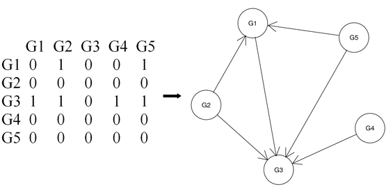
Figure 1. An example of adjacent matrix M and its corresponding directed acyclic graph G. M[i,j]=1 represents node Gj in G is a parent of node Gi in G. This network is generated from above bn.data example. G1~G5 corresponds to gene YAL022C, YAL040C, YAL053W, YAL067C and YAR003W, respectively.
To fully use our limited experiment data as far as possible, we generate several reasonable networks from microarray data perturbed by using Efrons non-parametric bootstrap approach with replacement. This procedure is implemented in the function BootstrapBN which takes bn.data and nboot (the times to bootstrap) as parameters:
> boot.ret <- BootstrapBN(bn.data, nboot)
boot.ret is an nboot-length list each of which element contains a network adjacent matrix reflecting the relationship of nodes in the network (Figure 1).
BootstrapBN produces several candidate 1st-order regulatory networks, which are further used to retrieve their meta-information to construct 2nd-order graph.
Reconstruct significant coherent regulatory modules
We extend CODENSE algorithm to directed graph. xCODENSE internally calls function HCS for mining Highly Connected Subgraphs.
Using xCODENSE, we could mine directed coherent sub-networks with high edge supports
> coh.dengraph <- xCODENSE (sumgraph.matrix, boot.ret)
coh.dengraph is an object with the type of list, each element of which is a sub-module retrieved from the network collection in boot.ret. For every coherent sub-network, we believe the feature and co-occurrence of all the edges in these modules are highly confident.
Remarks:
Currently HCS internally uses a graph-cutting algorithm minimum cut (function MINCUT) which is the fastest cut algorithm so far based on graph connectivity. In the upcoming version, for balancing the sizes of the resulting cut sets, we first call normalized cut algorithm (NCUT), and then when the sizes are reasonably small, we turn to MINCUT. NCUT function is already contained in the current version of BNArray, but the results do not show the stability. Thus, after improving implementation of the algorithm, xCODENSE can utilize the mixed cut algorithm to mine dense subgraphs.
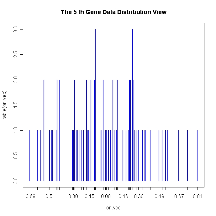
We can view the distribution of one genes expression level across all experiments, and the distribution of the gene expression levels in one microarray slide. For example, we want to observe the behavior of the 5th gene expression across the total 78 experiments, so we call function:
> EachGeneDataDistView(5,5,total.data$df.ori)
The sample image by using this function is showed in Figure 2.
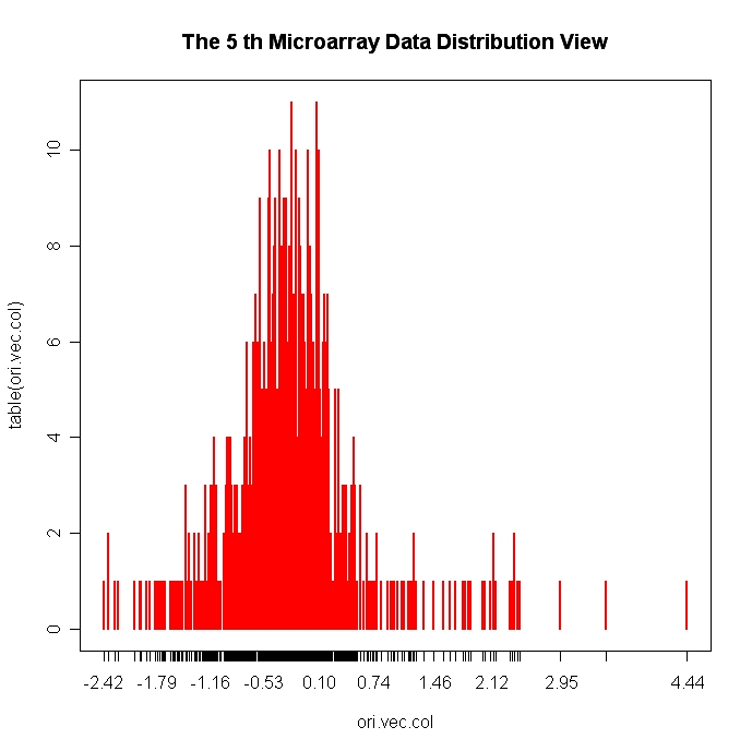
And similarly to view the distribution of expression levels of all genes in the 5th microarray slide, we use function
> EachMicroarrayDataDistView(5,5, total.data$df.ori, total.data$n.changed)
The sample image by using this function is showed in Figure 3.
Fig 2 and Fig3 give an overview of how the data approximately distribute for further statistical analysis and hypothesis tests.
To show how BNArray works, we can run the demo in this package (Spellman microarray data set)using the following command:
> demo(spd,package=BNArray)
Plots result after running demo:
Figures 4 --- A Bayesian network with the highest score
Figures 5, 6, 7 --- Bootstraped Bayesian networks with the highest scores (nboot=3)
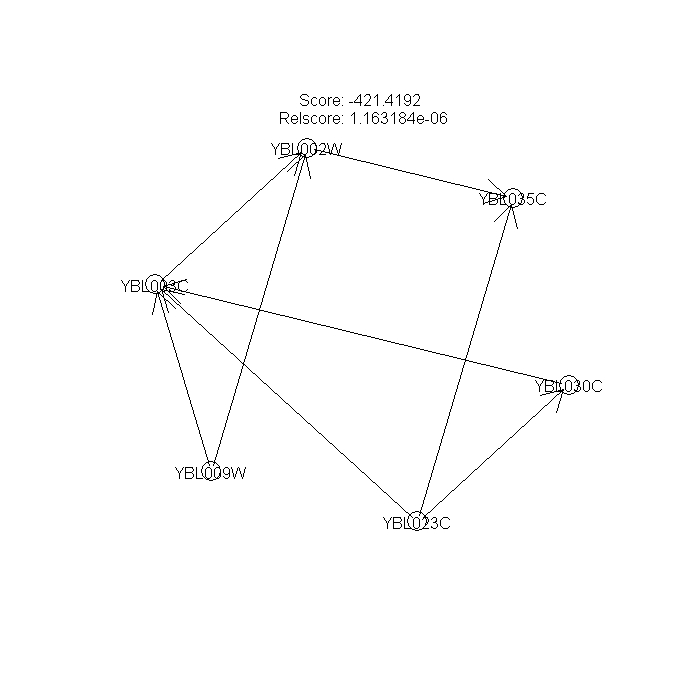
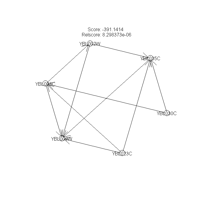
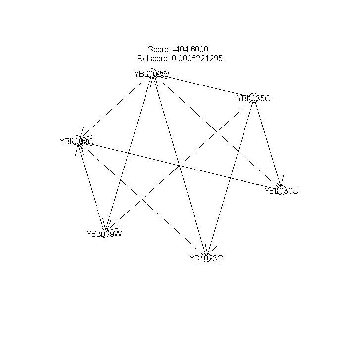
Figures 8 --- Summary graph from a collection of the 3 bootstrap-produced Bayesian networks
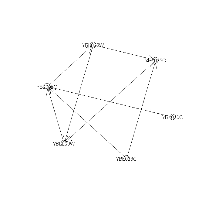
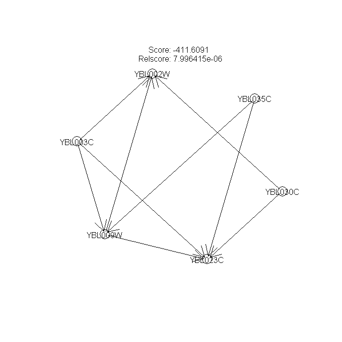
Figure 9 --- A significant regulatory sub-network mined from 1st-order networks
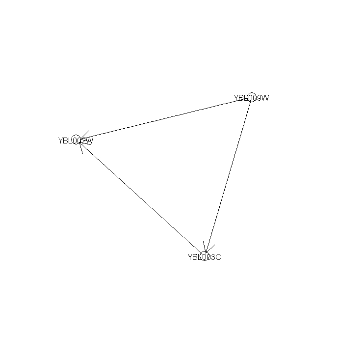
Discussions:
The results of Fig. 9 show that gene YBL009W (unknown ORF) co-regulates H2A (YBL003C) and H2B (YBL002W). H2A and H2B form a compound during DNA replication process. Checking the summary information about the function of YBL009W in SGD, we found YBL009W is a haspin which is involved in the meiosis process annotated in GO Biological Process database. This indicates that YBL009W is probably a co-regulator of H2A and H2B gene expression if it is not a component of the nucleosome.
Part II: Download & Utilization
Win32 binary code:
Linux source code:
Index of exported API functions:
Installation:
For installation in Linux, use command R CMD INSTALL /PKG_HOME/BNArray (/PKG_HOME is the home directory of package BNArray). For windows user, install the package from local BNArray*.zip file. Remember, before installing and using BNArray, make sure deal and dynamicGraph package has been installed.
We demonstrate BNArray on the S. cerevisiae cell-cycle gene expression data sets of Spellman et al (Whole microarray data set & differentially expressed gene names can be found here).799 differentially expressed genes are selected for potential further modeling. We selected genes involved in DNA repair from the 799 gene pool (17 genes).
We set the bootstrap times to 15, 30 and 45 for three experiments, respectively. The parameter of edge-connectivity threshold of highly connected networks has been set to 2/3*NodeNum of the network, and the threshold of the edge supports in the summary graph has been set to 1/2*nboot, 2/3*nboot and 3/4*nboot in three experiments respectively.
1. Out of the total edges in a complete network, 90% have the confidence below 0.67, which is the same for different number of bootstraps of 15, 30 and 45. This indicates that most of the edges in the induced Bayesian networks are extremely noisy (Fig 10). Thus, we choose the confidence level t=0.67 or t=0.75 for reconstructing coherent sub-networks. Moreover, most edges have confidence from 0 to 0.3. We can also observe that as the fold increases, the curve becomes smoother (Fig 11). However, the edges with confidence level from 0.9 to 1.0 are quite stable during the bootstrap approach, which suggests a strong relationship between these genes (see the table below). We order the confidence values of edges with their begin and end nodes in the summary network. The result is shown in the attached table.
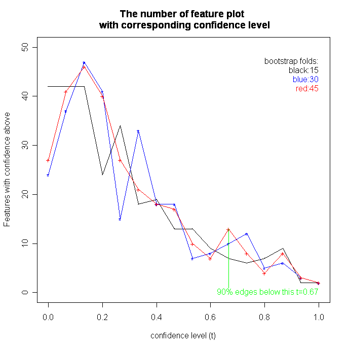
.png)
Bootstrap=15 | Bootstrap=30 | Bootstrap=45 |
"YDR097C" "YDL101C" | "YDR097C" "YDL101C" | "YDR097C" "YDL101C" |
"YIL066C" "YDL101C" | "YIL066C" "YDL101C" | "YIL066C" "YDL101C" |
"YKL113C" "YDL101C" | "YKL113C" "YDL101C" | "YKL113C" "YDL101C" |
2. An interesting phenomenon is that some genes (eg. YDL101C) tend to be regulated by many other genes, while other genes (eg. YKL113C) acting as dominant genes. These central genes may play a key role during the regulatory pathways or networks. Under the condition of nboot=45 and confidence level t=0.75, we can easily detect these high confident edge features (Fig 12). Also we could draw this result either from the attached table or from the reconstructed coherent sub-network (Fig 13).
.png)
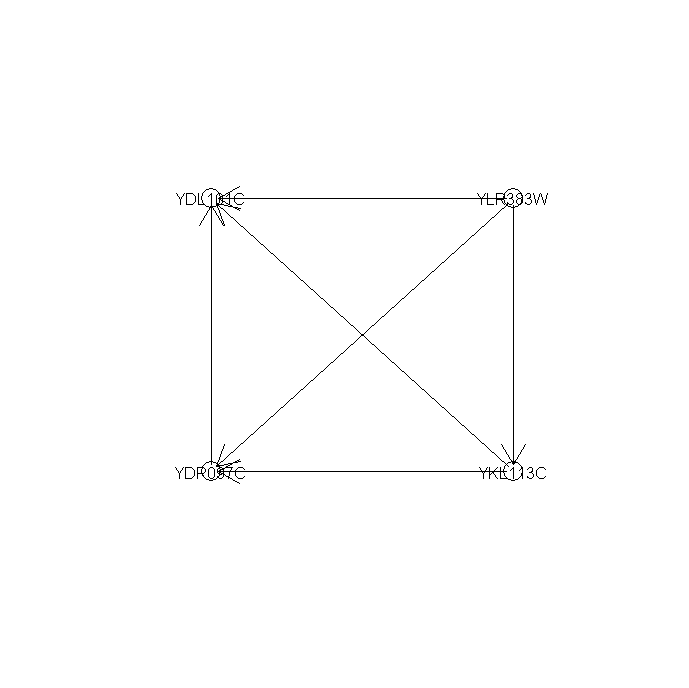
3. The dense coherent sub-networks mined from BNArray in this example with parameter nboot=45 and t=0.50 (Fig 13). This sub-network is recognized as a significant coherent module functioning as a group, either formed in a complex or genetic regulation relationship with other connected members in this group. From the summary database of SGD, we have consulted the literature concerning the relationship among the genes in this significant sub-network (1,2 etc.). As a result we found these genes involved in DNA repair are closely interacting in the above two forms.
Conclusion:
For fully interpreting the result, we can combine the results from summary graph and the dense coherent graph. We find this approach is quite cautious because the rate of false negative is high. This reminds us that the edges which do not have high confidence might be a correct edge.
1. James M. Bean, Eric D. Siggia and Frederick R. Cross (2005). High Functional Overlap Between MluI Cell-Cycle Box Binding Factor and Swi4/6 Cell-Cycle Box Binding Factor in the G1/S Transcriptional Program in Saccharomyces cerevisiae. Genetics Vol. 171, 49-61
2. Jana E. Stone and Thomas D. Petes1 (2006). Meiotic mismatch repair in S. cerevisiae. Genetics May 15.
Public research assisted by BNArray should cite this website and publication:
BNArray: an R package for constructing gene regulatory networks from
microarray data by using Bayesian network
Xiaohui Chen; Ming Chen; Kaida Ning
Bioinformatics 2006; doi: 10.1093/bioinformatics/btl491
Maintainer: Xiaohui Chen E-mail: cxh1984@interchange.ubc.ca Last updated: 2006/09/27