1.     Framework

With the rapid development of high-throughput sequencing technologies, the amount of biological data is growing exponentially. The Soybean Omics Database (SoyOD) is a newly developed multifunctional database integrating multiple omics datasets and interactive analysis tools made available to aid soybean molecular research and breeding. SoyOD collects in one place the most complete set of soybean genome data available, comprising 6 telomere-to-telomere (T2T) assemblies and 53 chromosome assemblies. In addition to the published sequencing data, 984 newly sequenced, high-depth soybean accessions were included, which contained 5,685,352 SNPs and 1,361,946 InDels. Another ~4000 re-sequenced soybean germplasms from public data sources were also integrated into SoyOD, generating 7,193,573 SNPs and 753,361 InDels. SoyOD also contains 14,977 records of 225 different phenotypes, including plant architecture, biochemistry, plant growth and development, yield, and abiotic and biotic stress traits. The transcriptomic data represents 1097 different tissues and varieties, discreet tissues within seeds during different stages of development, and samples undergoing abiotic or biotic stress or during nutrient absorption. The SoyOD is divided into six basic modules, namely the genome, phenome, population, transcriptome, variome, and synteny modules. An additional toolkit is provided to facilitate access and processing of data that includes Jbrowse, BLAST, a soybean genome version converter, a sequence extractor, an expression heatmap generator, a diversity viewer, and a haplotype viewer.

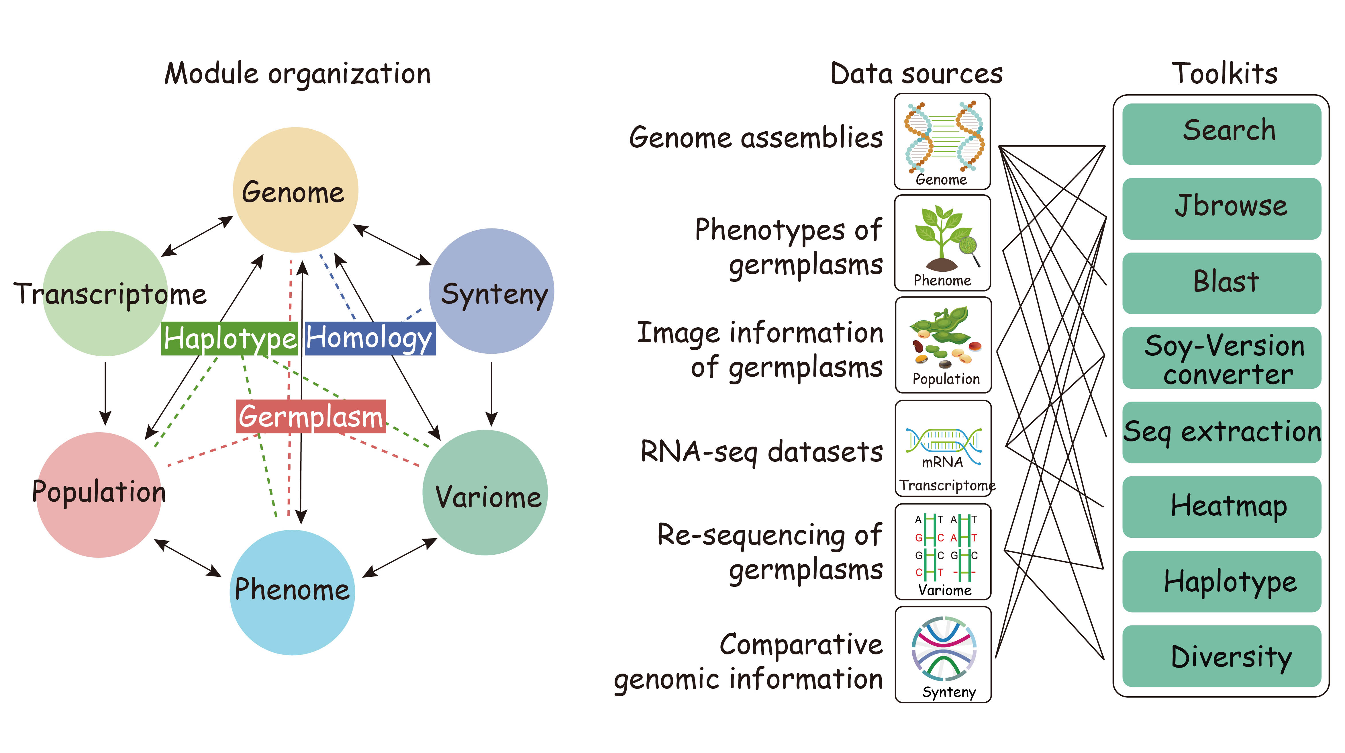
Fig. 1. Functional overview of the Soybean Omics Database (SoyOD) hosted at https://bis.zju.edu.cn/soyod/home/.

2.      Search

The easily accessible search interface includes a multifunction search bar that can handle different input types (some example text strings shown below bar):

Ø  All, global search for complete or incomplete keywords.

Ø  Genome, search for the 59 different genomes by name.

Ø  Gene ID, search by gene ID.

Ø  Region, search by chromosome number with start and end positions.

Ø  Germplasm, search by complete or incomplete variety name or number.

Ø  Phenotype, search by phenotype (full name and abbreviation) or ID.

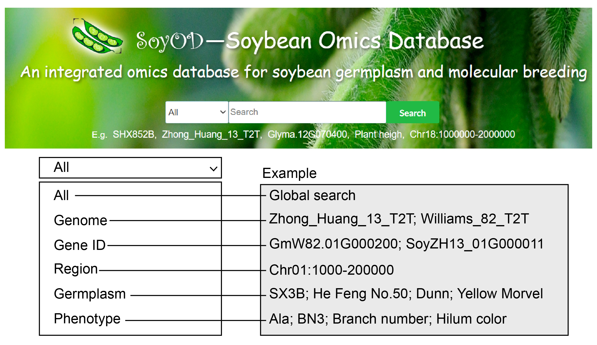
Fig. 2. Easy-to-access search interface that can accept multiple types of inputs.

3.      Genome

The genome module contains six submodules, namely Genome assembly, Gene browser, Gene search, Transcription factor, Transposable element, and Homologous gene.

3.1   Assembly genome

The genome module contains the information of 59 De novo assembled genomes, including chromosomal level 6 wild soybean from G. soja, 31 improved cultivars and 10 landraces from G. max; 6 from perennial Glycine spp., 6 T2T level genomes. Meanwhile, the assembly level, chromosome length, chromosome density, accession information and de novo assembly statistics can be found in the genome assembly submodule. In a lower window, the gene density for each genome can be viewed.

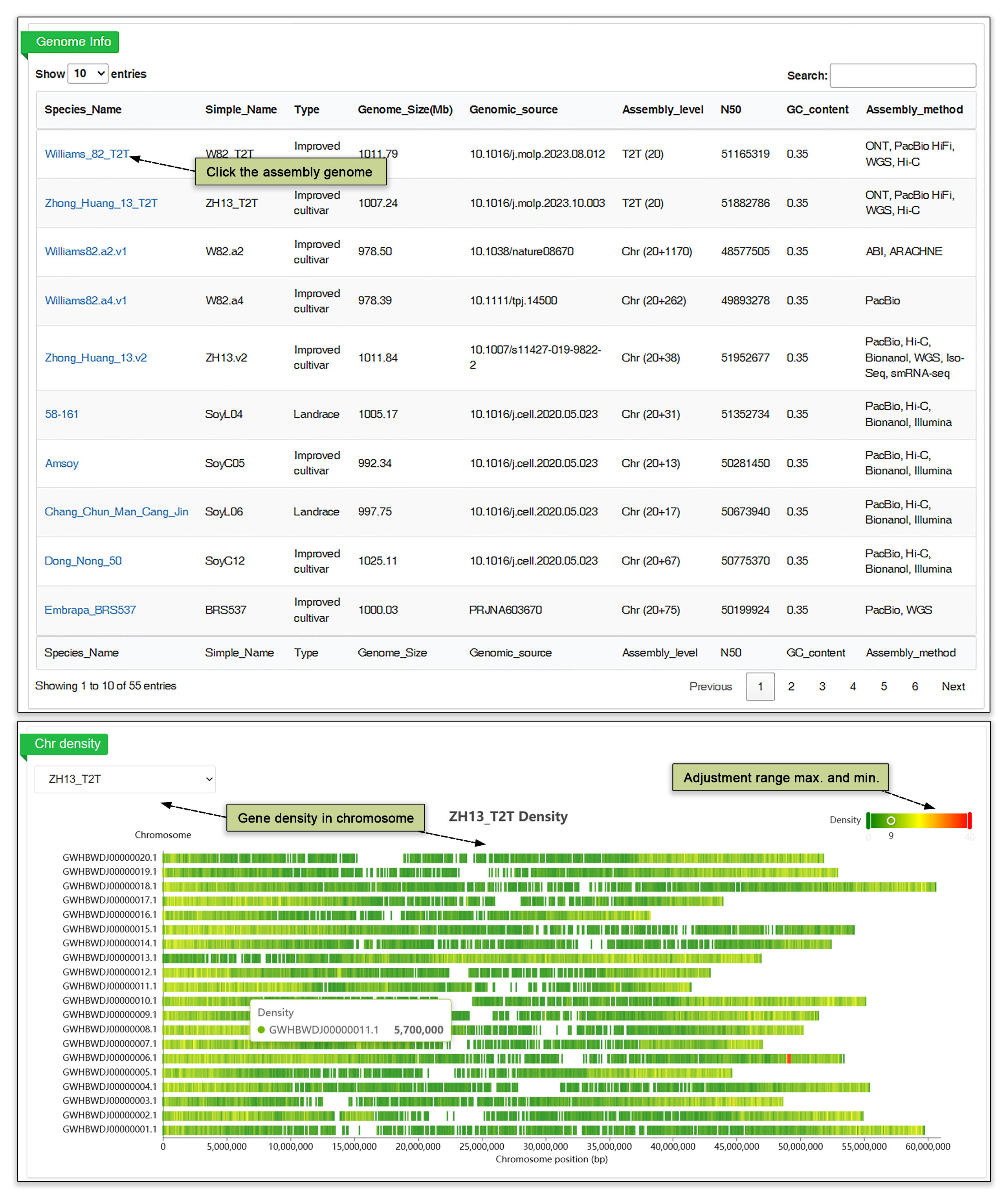
Fig. 3. Genome Assembly information and gene density viewer.

3.2   Genome browser

In the genome browser submodule, users can select a genome, organized by landrace and cultivar of annual soybean and by wild perennial species. Clicking on any genome assembly will call up the list of identified genes by gene ID as well as each gene’s chromosomal position, strand, and a description.

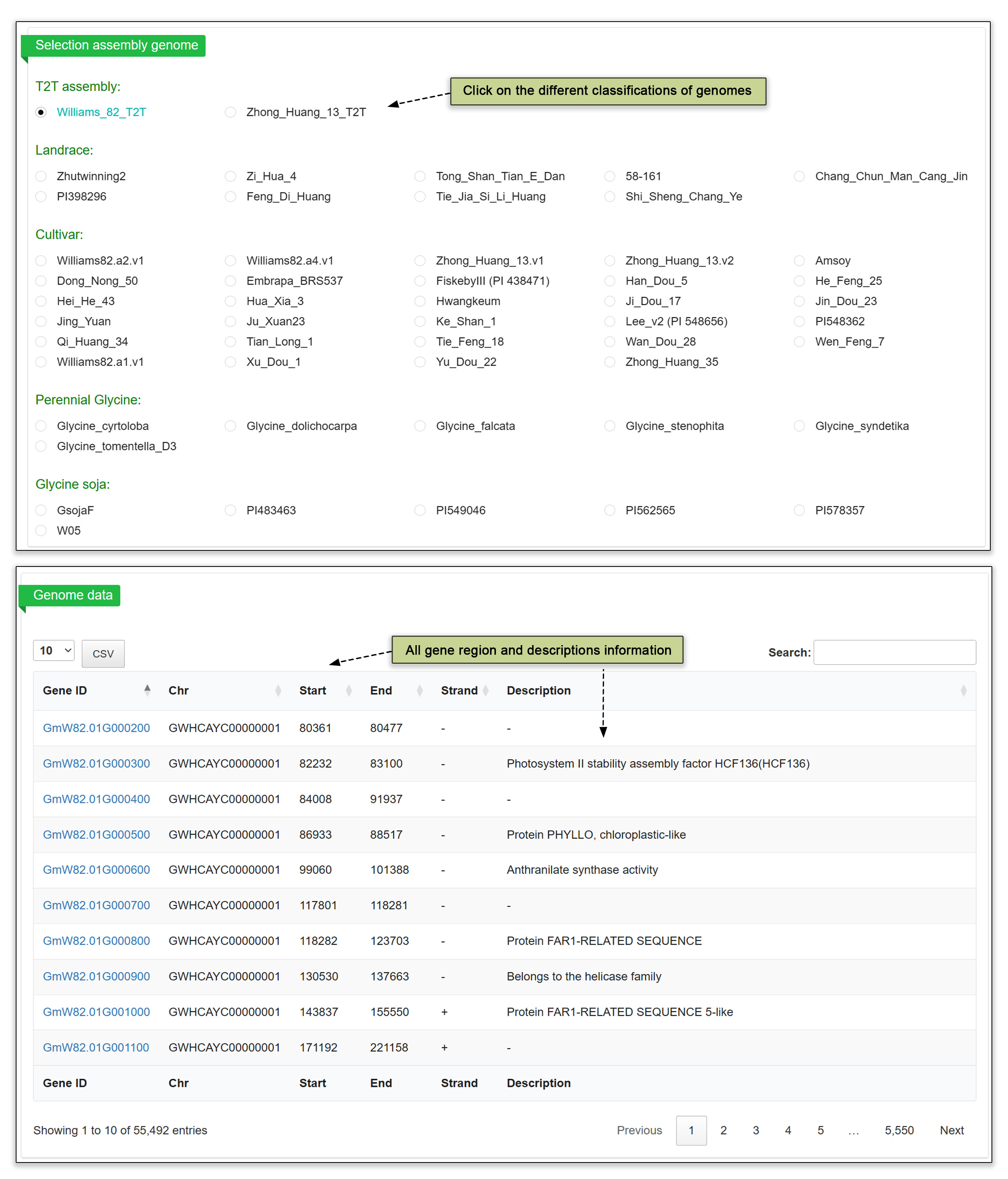
Fig. 4. Genome browser submodule.

 

3.3   Gene search

In the gene search submodule, users can input multiple gene IDs without any additional distinguishing genomic information to obtain a table of genes. clicking on gene ID opens a page containing basic gene information, a gene structure view in JBrowse, the in silico translation sequence, GO/KEGG annotation and any QTLs.

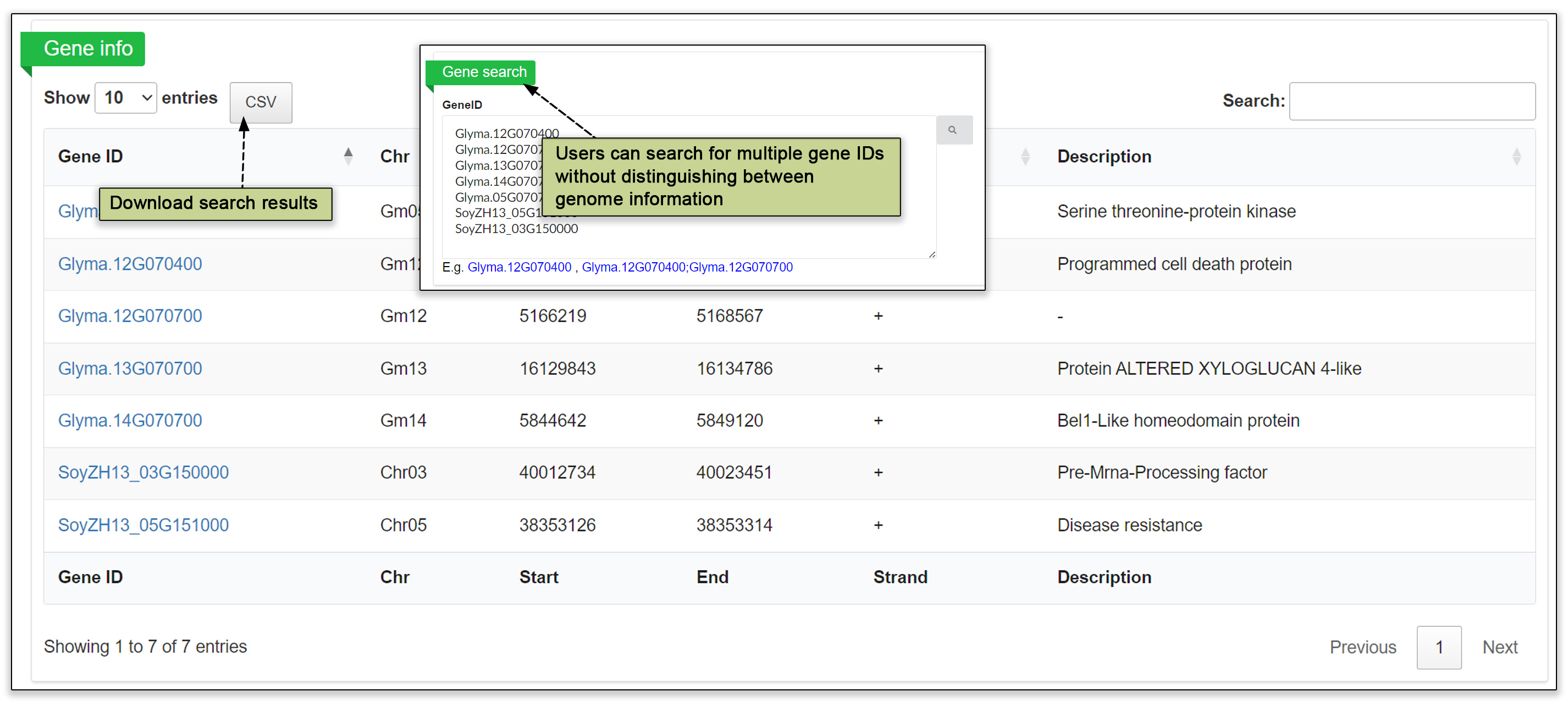
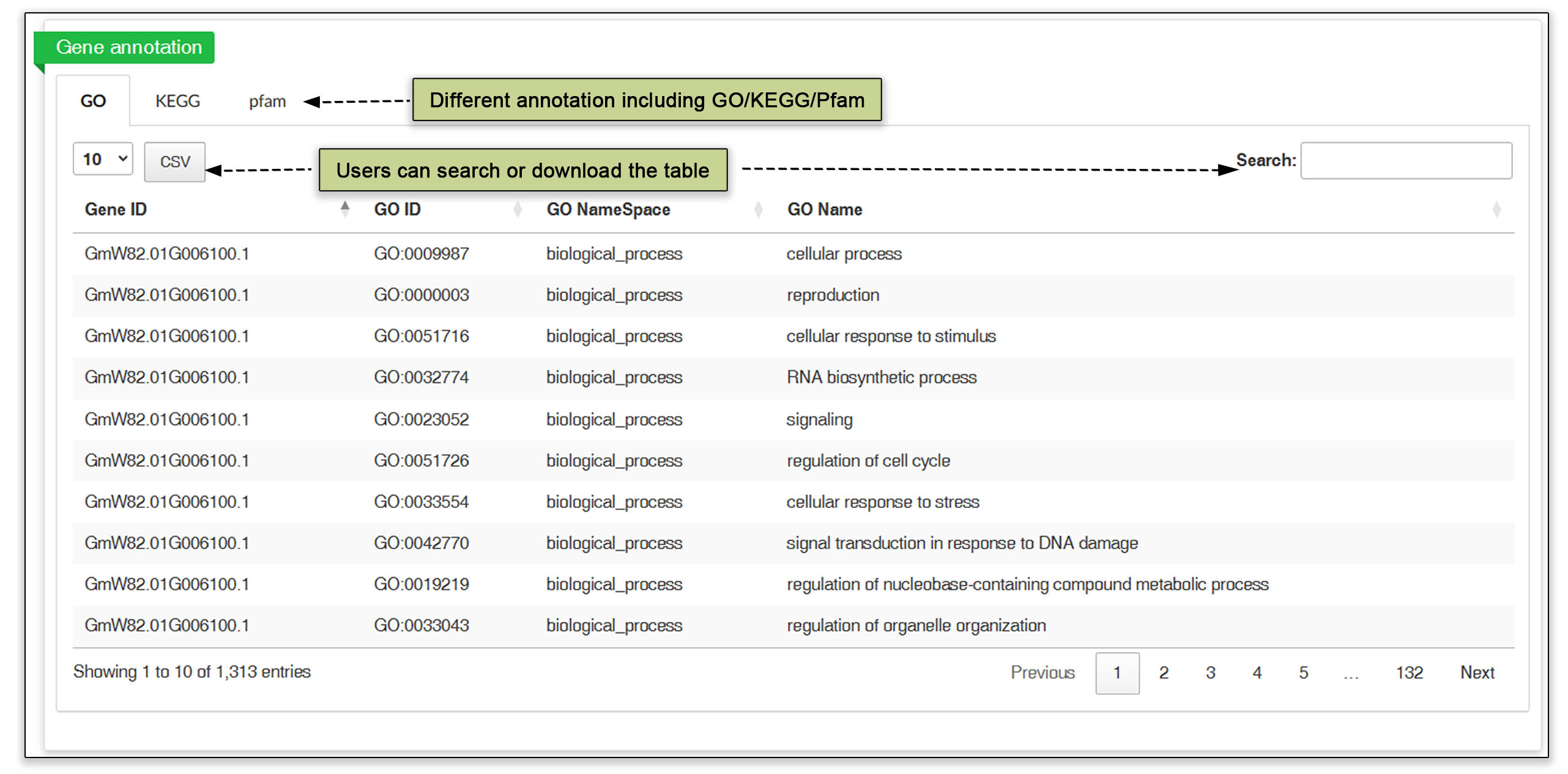
Fig. 5. Detailed information about a gene obtained by searching by gene ID.

3.4   Transcription factor (TF)

In the transcription factor submodule, the transcription factor information from the Arabidopsis genome was used to predict the corresponding soybean transcription factors by protein sequence comparison followed by annotating the genes encoding these transcription factors. Users can view the number of genes predicted in all gene families by each assembled genome or view each TF family by genome.

 

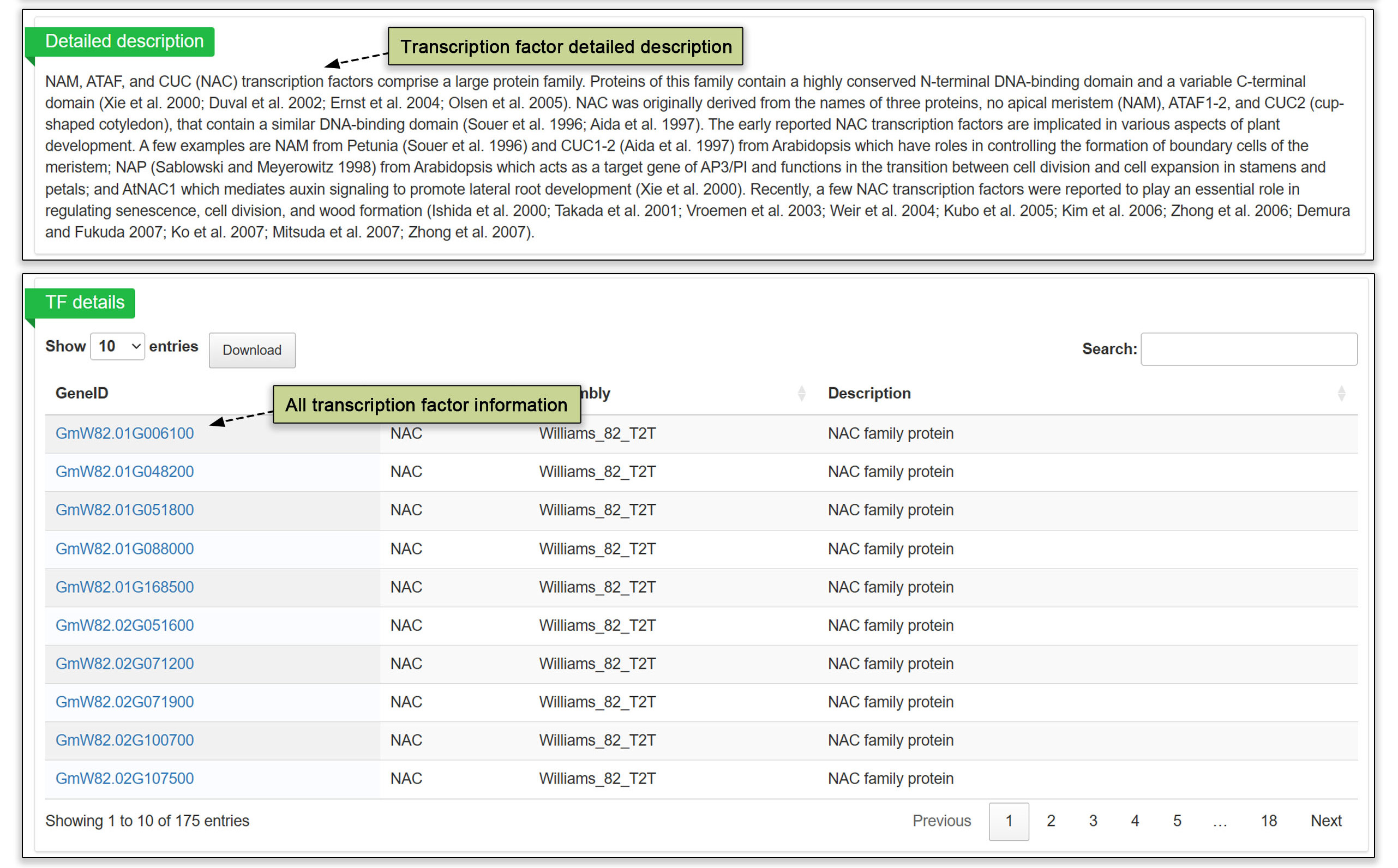
Fig. 6. Transcription factor submodule with TFs predicted based of Arabidopsis protein sequences.

3.5   Transposable Element (TE)

The transposon submodule contains a radial graph of the proportion sequence that is either non-TE or one of 15 classes of TE within each of the 59 genomes. and classifications. Additionally, users have the option to search by chromosome region or TE family for the corresponding transposon information.

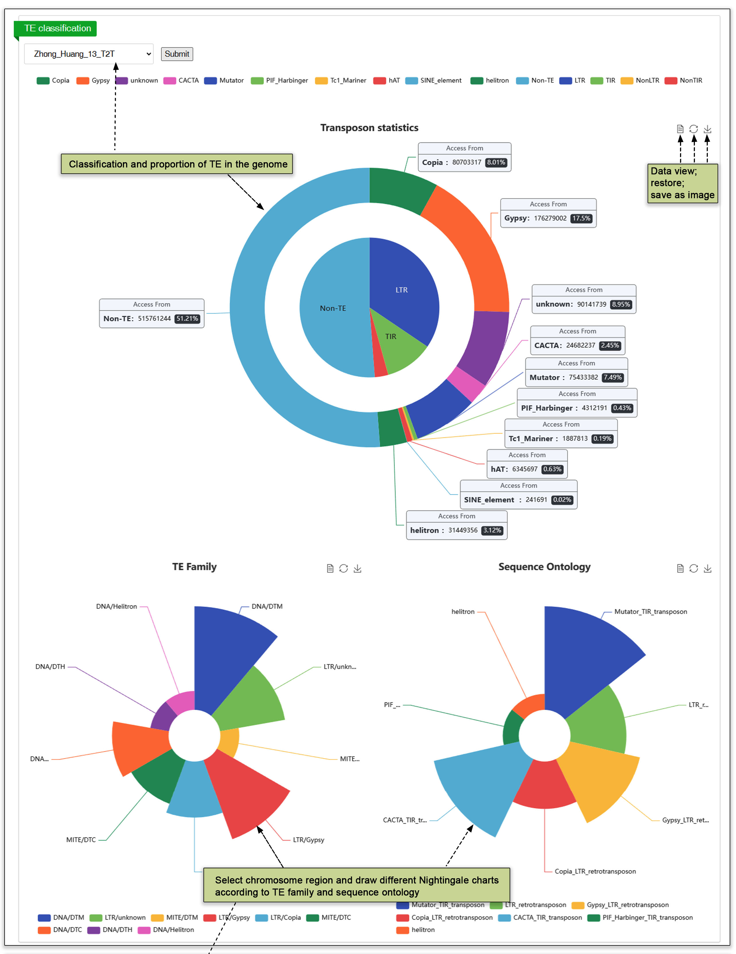
Fig. 7. Transposon search.

3.6   Homologous genes

Orthologous data is readily accessible, allowing users to input either a gene ID or a homologous group code to retrieve a list of potential homologs across the different genomes. The total number of predicted genes for each homologous group is listed in the upper table. This feature streamlines the process of comparative genomic analyses and facilitates the study of evolutionary relationships between genes in various accessions.

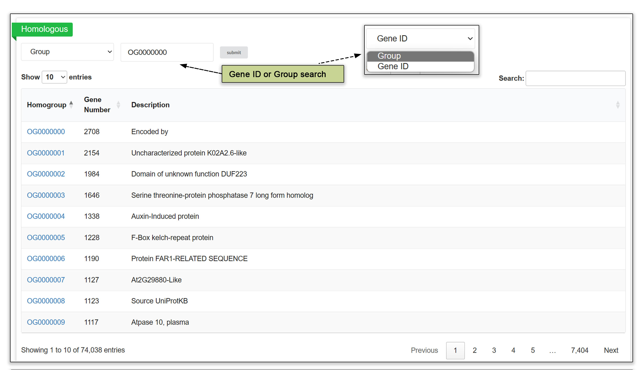
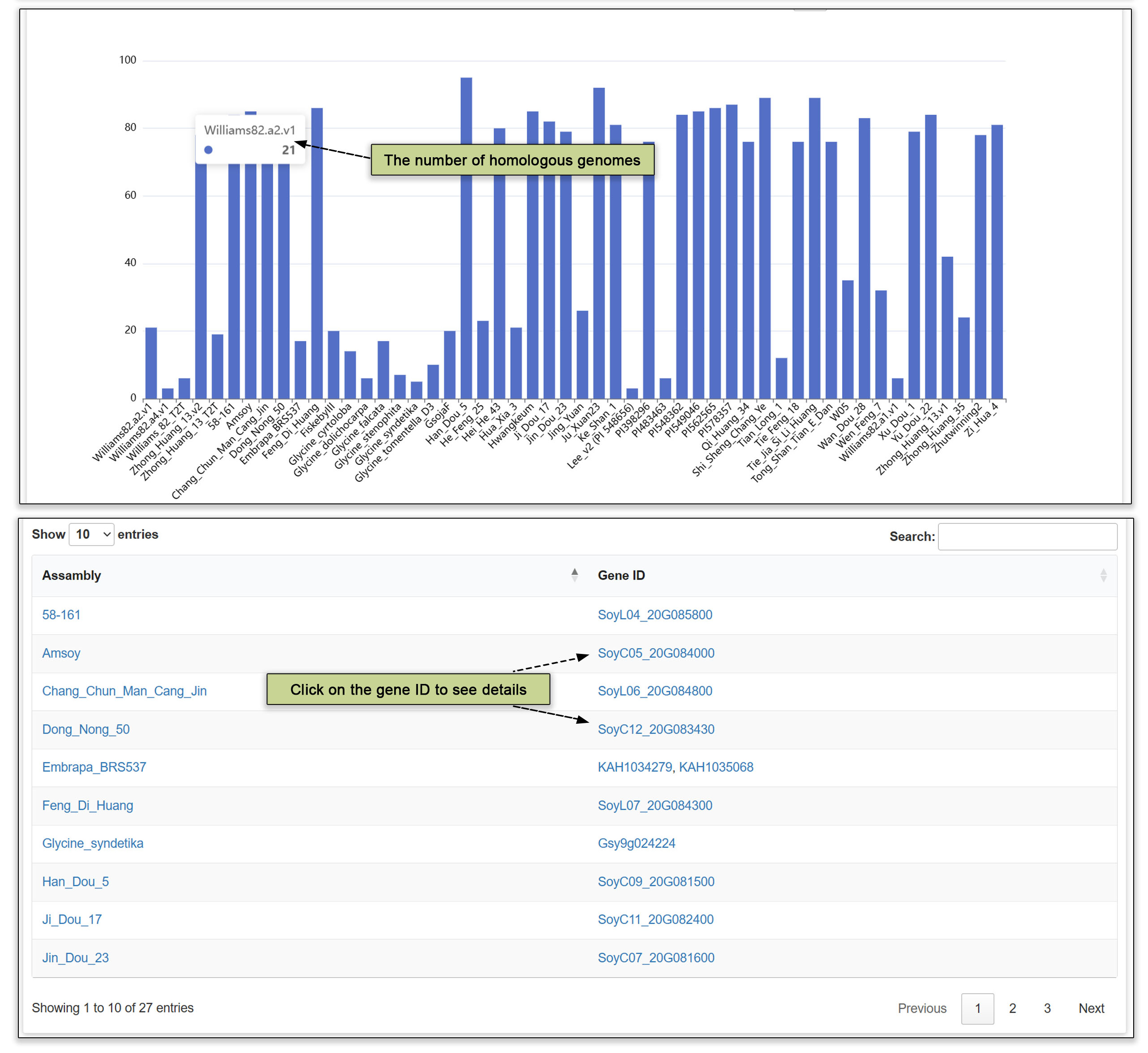
Fig. 8. Homologous genes submodule.

4.      Transcriptome

The Transcriptome Module contains gene expression profiles from a total of 1097 RNA-seq libraries. These datasets were integrated into 8 submodules (that can be searched through visuals), including tissue expression and seed development tissues (illustrations of plants), tissue and seed development expression across accessions (heat maps), during abiotic and biotic stress and nutrient absorption (illustrations of plants) and co-expression (through a network map). We set up five representative genomes, including the two most recent T2T-level genomes (Williams 82 T2T and Zhonghuang 13 T2T) and three commonly used chromosome-level genomes (Williams 82 v2, Williams 82 v4 and Zhonghuang 13 v2) as reference genomes so that users can easily access the gene expression level by entering the corresponding ID.

4.1   Tissue expression

In the tissue expression module, a soybean electronic fluorescent pictographic (Soy-eFP) and a suite of other interactive tools enable users to comprehensively view gene expression levels in tissues at different stages of development. We provide two divisions, one that includes expression across 27 tissues in Zhonghuang13 and Williams 82 and another that includes the expression across 9 tissues from 26 accessions. Searching for a gene in this module returns a gene table, bar chart, heatmap and line chart displaying the FPKM, TPM and Count values in the available tissues.

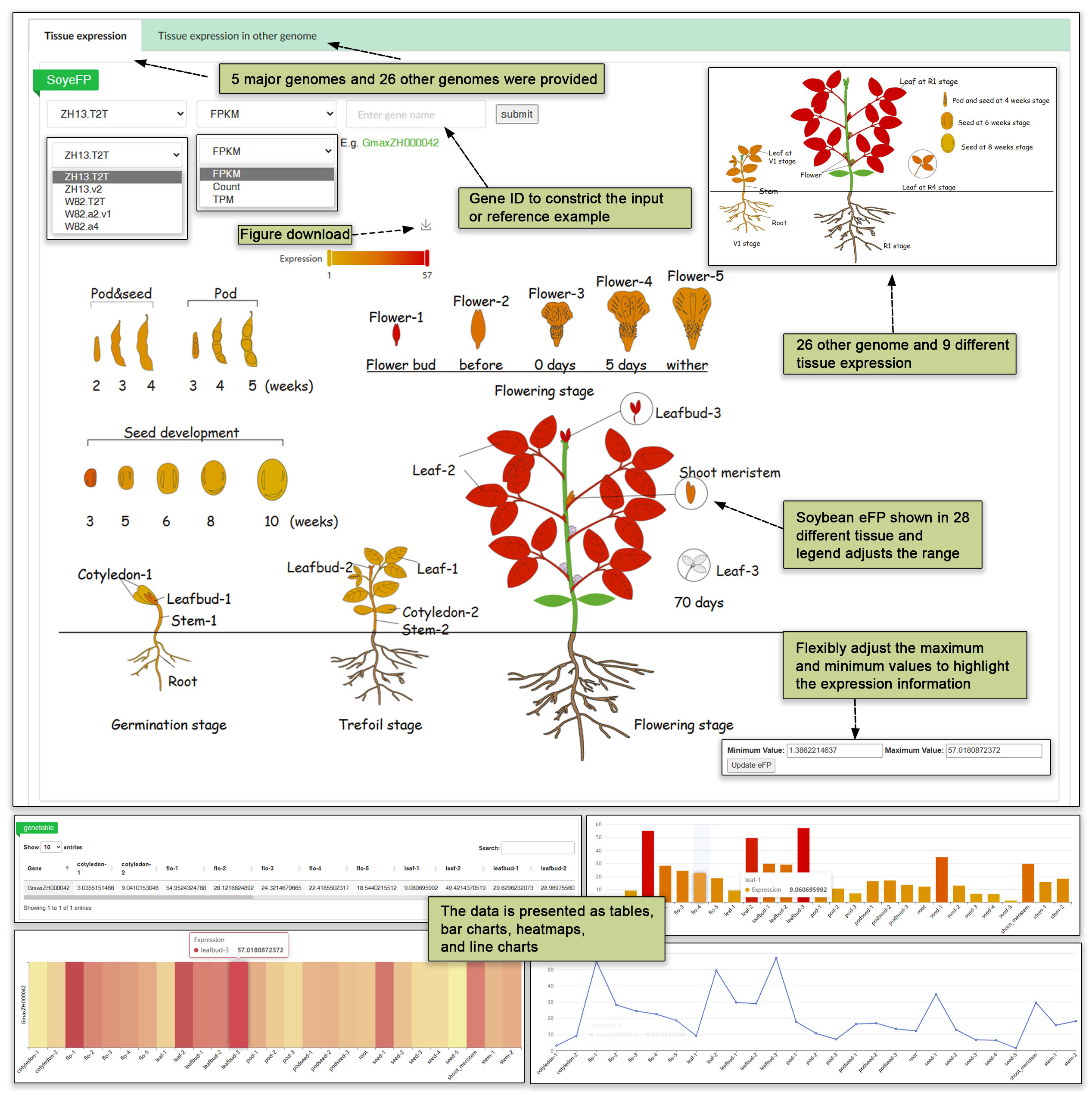
Fig. 9. Tissue expression across 31 genome assemblies with various visual representations.

4.2   Seed development subregions

We integrated expression data from 297 soybean accessions during four stages of early seed development sampled by laser capture microdissection (LCM) (Pelletier et al., 2017). To The SoyeFP visualizer included diagrams of seed slices across four stages of development that facilitates observation of gene expression.

Fig. 10. Seed development subregions dissected using laser microscopy. These slices were transformed into eFP visuals within SoyOD (Pelletier., 2017).

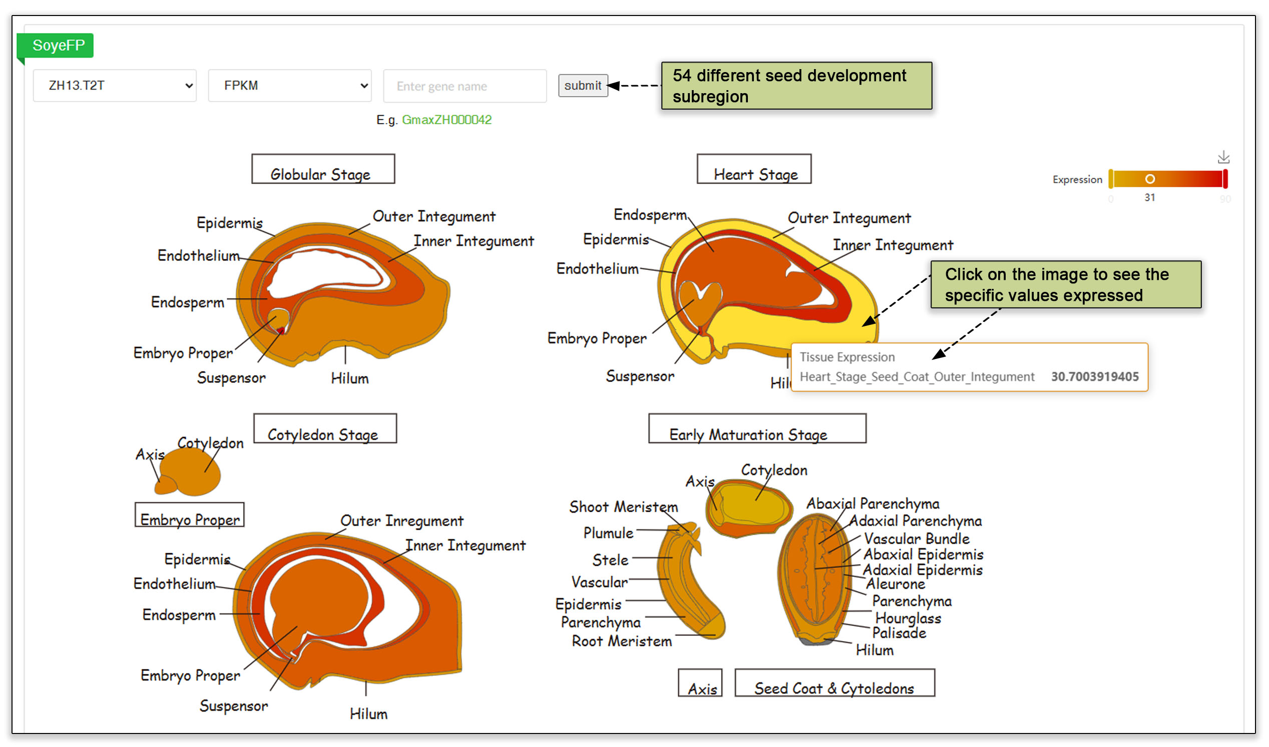
Fig. 11. Outline of discreet tissues during seed four stages of development, namely the globular stage, the heart stage, the cotyledon stage and the early maturation stage.

 

4.3   Tissue expression and seed development in germplasm

Two submodules are available to search for gene expression in different germplasm, at the tissue and seed development levels. Clicking on one of these submodules and searching by a Gene ID yields an expression heatmap across tissues using one of five reference genome assemblies. This tailored approach pinpoints the activity of a gene of interest under diverse conditions. The heatmap can use FPKM, Count, or TPM data. The module presents gene expression levels across the population of accessions, which can be useful in phenotypic studies and breeding efforts.

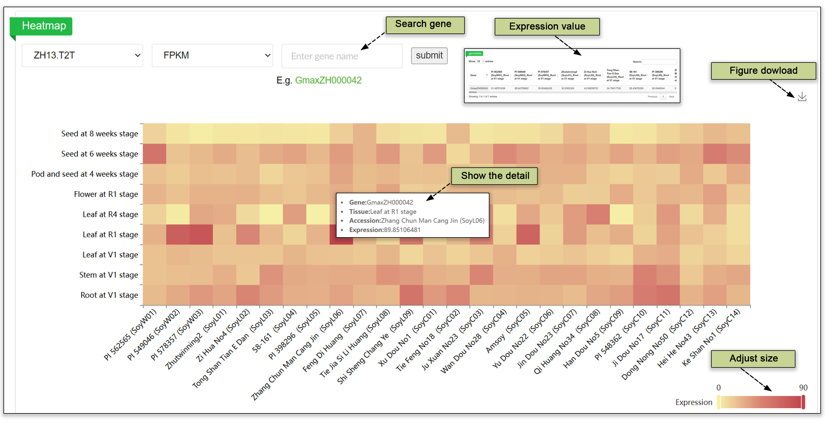
Fig. 12. Heatmap showing tissue expression and seed development across the germplasm resources.

 

4.4   Abiotic, biotic, and nutrient stress submodules

To further enrich exploration of the expression data, and thereby expand our understanding of plant resilience and adaptation, we developed additional transcriptome submodules focusing on biotic stress, abiotic stress, and nutrient uptake using eFP visuals. A Gene ID can be searched against abiotic, biotic, and nutrient stress conditions, including 11 abiotic stress conditions, fungal, bacterial and viral pathogen challenges, and sufficient and deficient conditions for 5 nutrients.

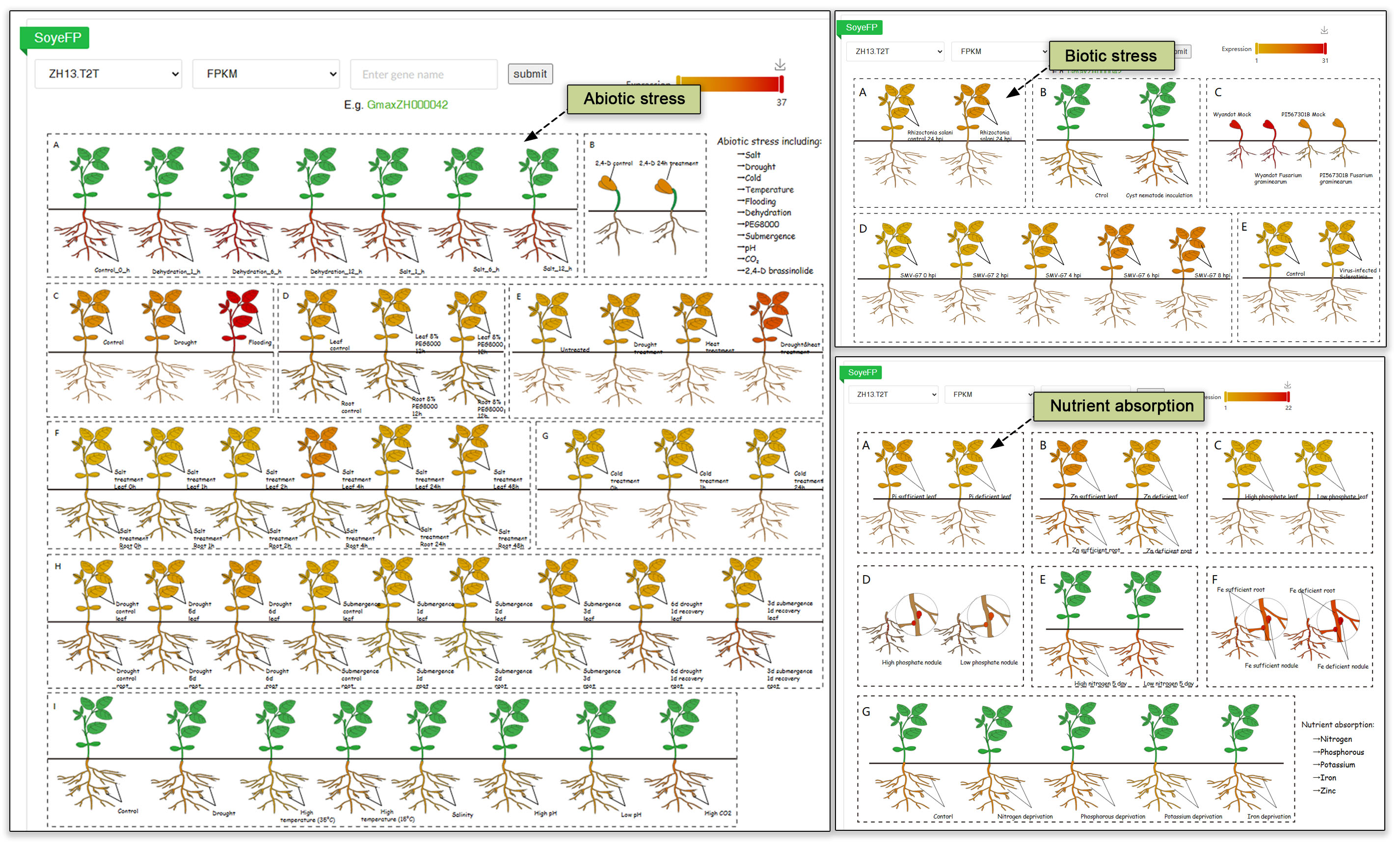
Fig. 13. Transcriptomic analysis in different abiotic, biotic, and nutrient stress conditions.

 

4.5   Co-expression submodule

A co-expression network is a visual representation of gene expression data that illustrates the relationships between genes based on their expression patterns. This type of graph can help identify clusters of genes that are co-regulated or functionally related, providing valuable insights into gene networks and biological processes. Users can enter one or more gene IDs into this submodule to query the co-expression network.

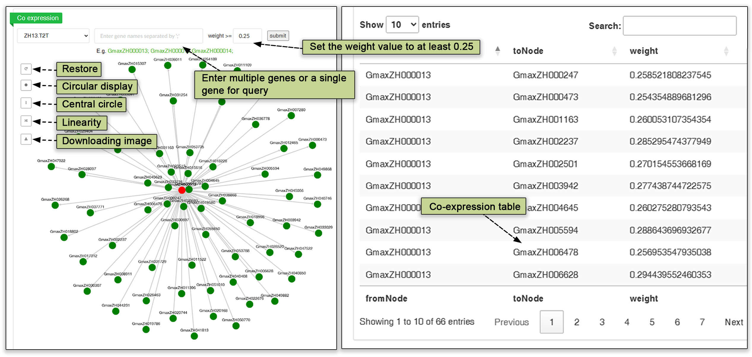
Fig. 14. Co-expression network graph and table of interacting genes.

 

5.      Phenome

The phenome module contains eight submodules, namely a germplasm search, viewers for traits and geography of the germplasm (called germplasm distribution) and links to quickly view traits related to a few phenotypes, namely plant architecture, biochemistry, plant growth and development, yield, and abiotic and biotic stress responses.

5.1   Germplasm search

The germplasm search submodule contains a set of harvest-stage and seed images, as well as information on more than 4097 accessions. The image database can be searched by name or ID. The germplasm search can be used to sort local (from lab obtained) and public (from Liu et al, 2020) germplasm resources by name, species, population, country of origin and even publication reference (first author last name). The germplasm table can be sorted by headline. This submodule provides key phenotypic information in a single view.

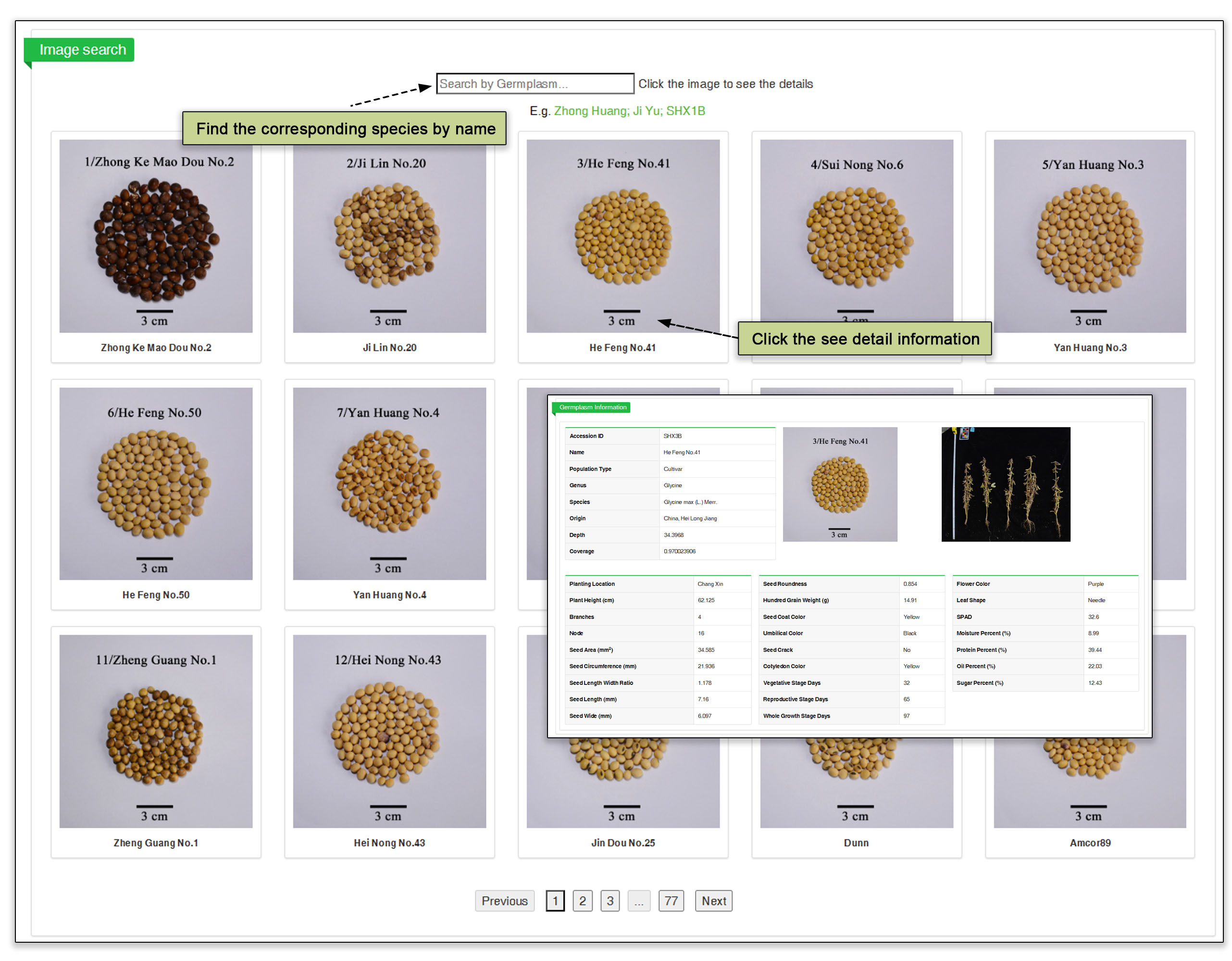
Fig. 15. Overview of germplasm resource submodule.

5.2   Germplasm distribution

In the germplasm distribution submodule of the Phenome module, 225 phenotypes are categorized into a 3-level catalogue based on obtained records. Users benefit from the convenience of swiftly selecting a phenotype by interacting with the sunburst graph. Once a user has found a trait ID of interest, users can search or find the tables detail information. A click in the center of the sunburst returns the burst graph back up one level. The phenotype records are initially classified using different qualitative tags or quantitative value regions. A second view in this submodule is a map of the origins of each soybean accession within the database. The map can be viewed globally or just for China, the center of origin of soybean.

Fig. 16. Phenotypic classes and geographic distribution.

5.3   Phenotypes submodules

The next submodules under phenome are upper-level phenotypic categories, namely plant architecture, biochemistry, plant growth and development, yield, abiotic stress, and biotic stress. Within the upper-level categories are 30 second-level subclasses, which can be viewed and sorted in the table. A used can find a trait ID in the Phenotype Class sunburst (Section 4.2), then search it in the Phenome table. The 30 trait subclasses are seed weight, whole plant morphology, seed morphology, flower morphology, leaf morphology, moisture content, oil content, protein content, growth morphology, sugar content, whole yield, lodging incidence, fatty acid content, trichome morphology, iron-deficiency, mineral and ion content, pod number, pigment content, fatty acid component, amino acid content, root nodule morphology, fruit morphology, animal damage resistance, microbial damage resistance, stem morphology, UV-B radiation, drought, electrical, root morphology and plant vitality. Clicking on a trait ID opens a second table further down the webpage, which lists the phenotypes that can be obtained by searching or sorting. The third graph shows the distribution of the range of values measured for this phenotype in our trials.

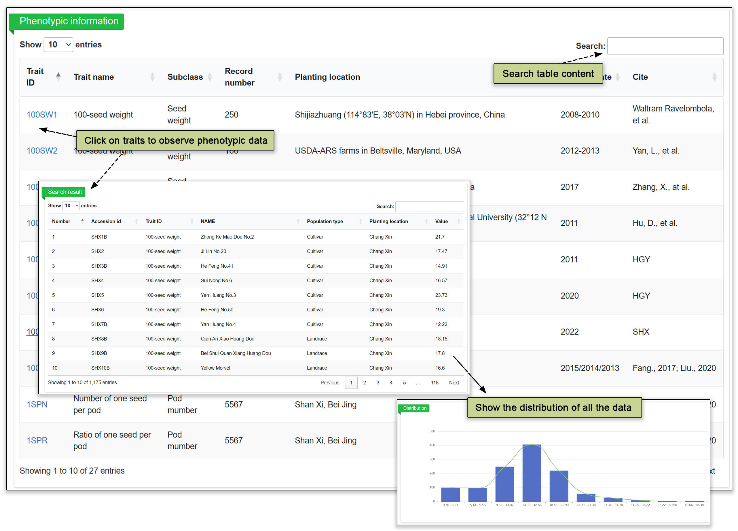
Fig. 17. Phenotypic classification and specific information.

 

6.      Population

The Population Module contains information on the 3904 accessions that have been sequenced. Among these resources are 940 accessions that our group re-sequenced fort his database. The newly re-sequencing set can be browsed or searched separately or with the published re-sequencing sets. The table can be sorted by genus, species, type (cultivar, landrace), accession name, or origin.

6.1   Population selection

The population selection submodule contains data from extensive selective sweep analyses of the high-depth sequencing data (984 accessions) and of all varieties data (3904). Four different analysis methods, FST, pi ratio, XP-CLR, and Tajima’s D, were employed for the whole genome selective test. Users have the flexibility of zooming in on regions of interest using a slider at the bottom or by searching chromosomal location, with the top 5% threshold represented by a dashed line. Figures of the selective sweep are available for download. Comparison plots can be removed for a clearer view of the sweep.

 

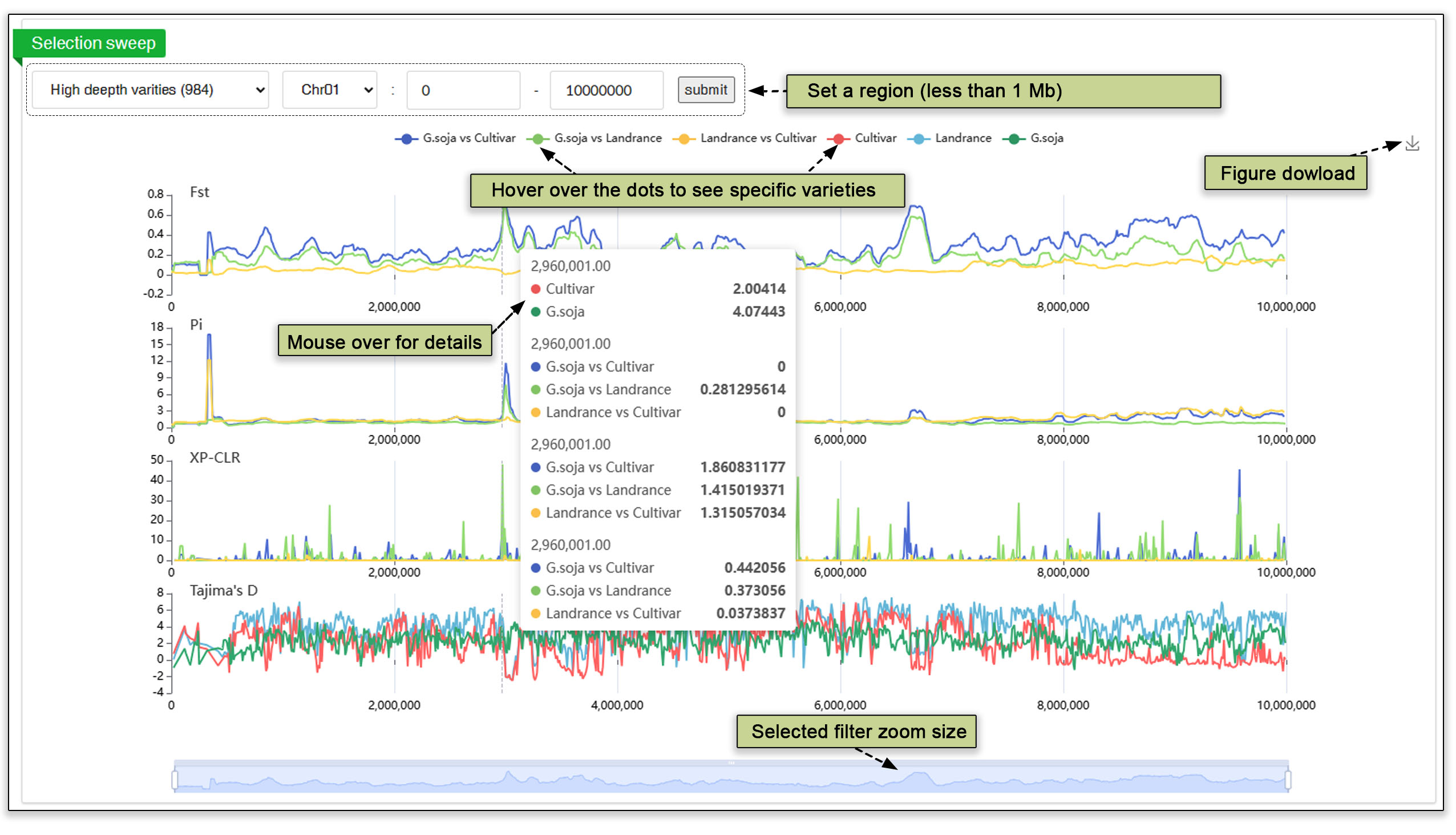
Fig. 18. Selective sweep analysis at the population levels.

6.2   Population structure

The population structure submodule contains principal component analyses, a population structure, and an evolutionary tree. These analyses help users gain a deeper understanding of group dynamics within populations.

 

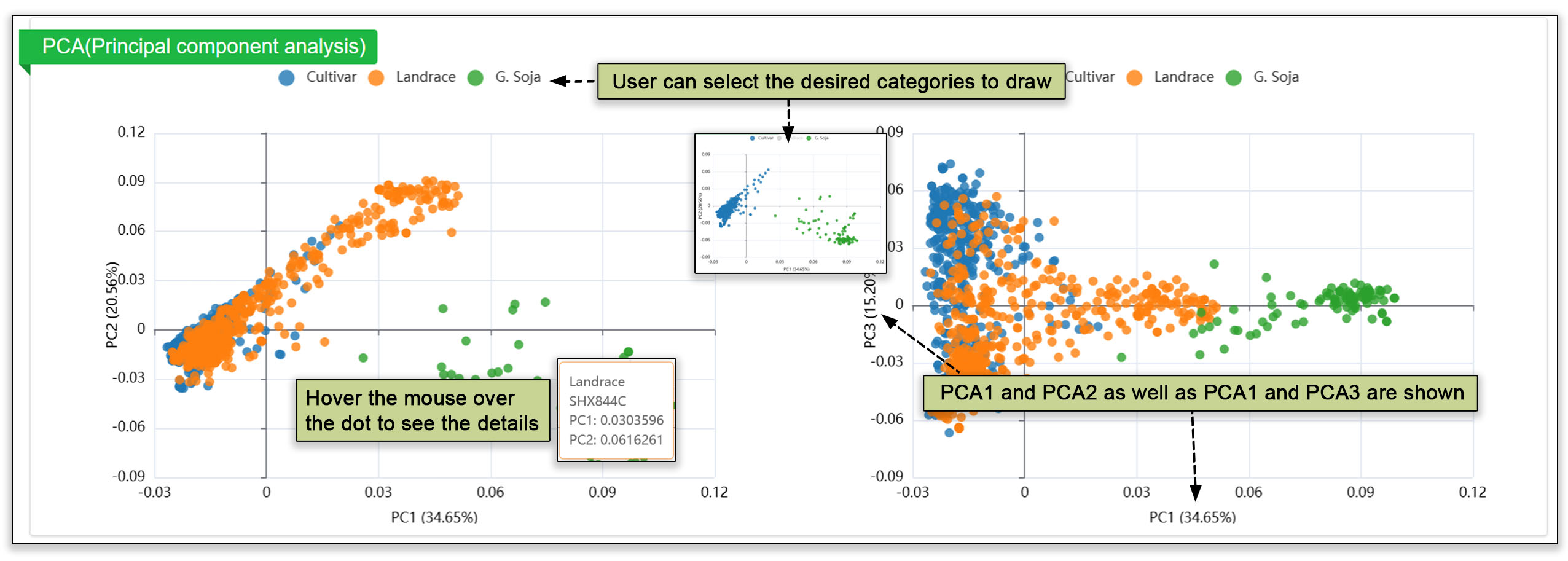
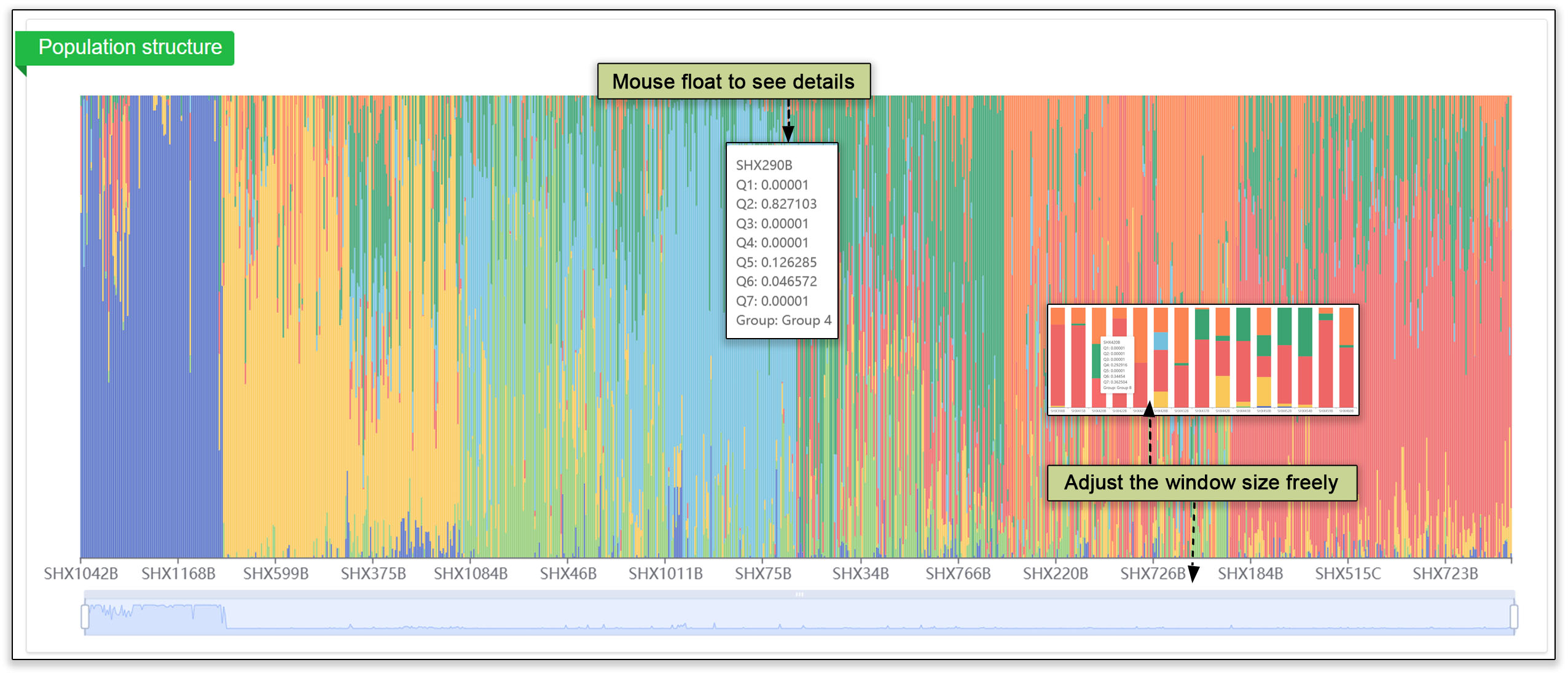
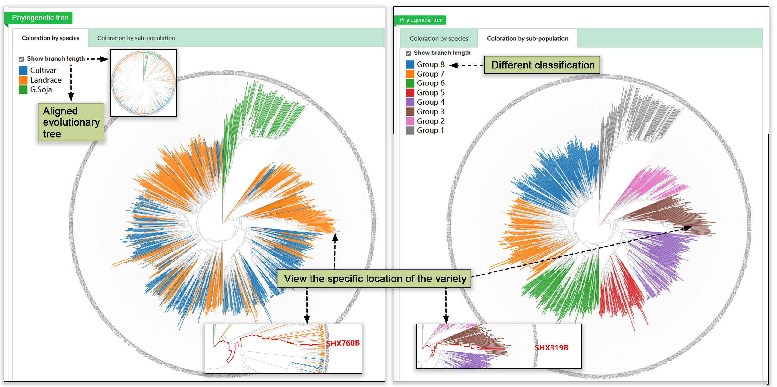
Fig. 19. Analysis of the populations by principal component analysis (PCA), population structure overview, and evolutionary tree.

 

7.      Variome

7.1   SNP and InDel

The densities of SNPs and InDels can provide insight to the genetic variability within organisms and identify genes with variable alleles within a population. A user-friendly interface has been developed to enable users to efficiently search between chromosome regions to find variant across 3904 accessions.

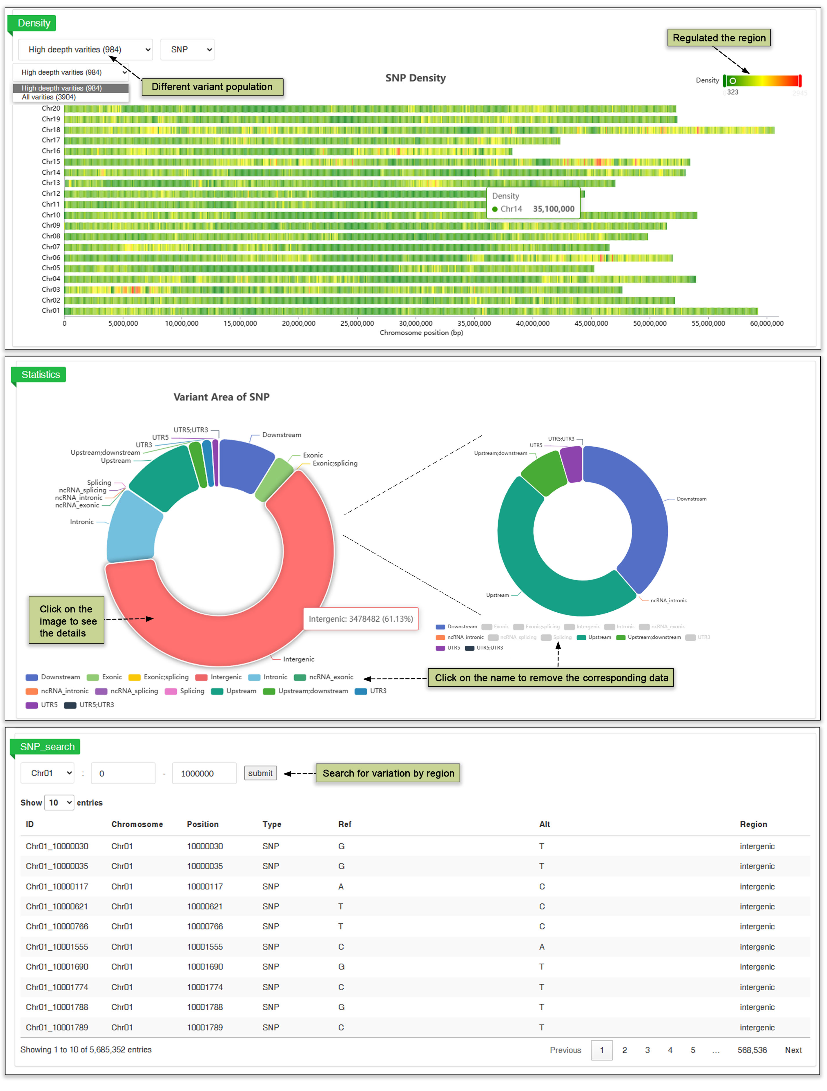
Fig. 20 Variation browser

7.2   GWAS

In the GWAS submodule, the user first clicks on a phenotype name to view associated genomic locations for that phenotype. The first graph is a Manhattan map (of 0.5 Mb windows) in which the p-value of each window is the p-value of the most significant SNP. The user can zoom in or out by scrolling the slide bar below the graph. The user can then click on bars with high p-values to see a table of significant SNPs in that area, along with the corresponding GWAS statistics and the Manhattan plot.

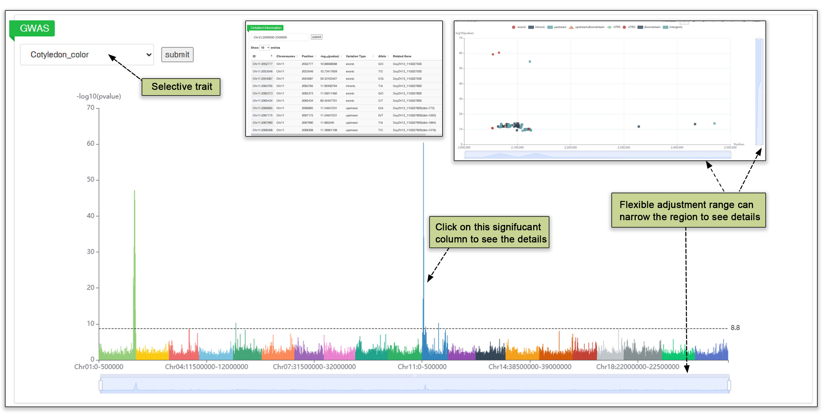
Fig. 21. Genome-wide association analysis of SNPs.

8.      Synteny

The synteny module includes a comparative genomic analysis of the 52 assembled genomes. The genomic collinearity between the Zhonghuang 13 v2 reference genome and a genome of choice can be viewed in the embedded SynVisio web service, while genome variation can be browsed in genome and dotplot views.

8.1   Synvisio

Initially, the McScanX software will allow researchers to generate two main types of files: Genome Comparison GFF and Chromosomal Collinearity files. This step lays the foundation for the entire analysis process. Using these generated files, users can then easily identify and analyze areas of collinearity between different genomes. This is important for revealing evolutionary relationships between accessions and conserved regions within genes. Visualization using the genome comparison and collinearity files generated by the SynVisio software allows users to find genomic synteny and dotplot results for relevant chromosomes.

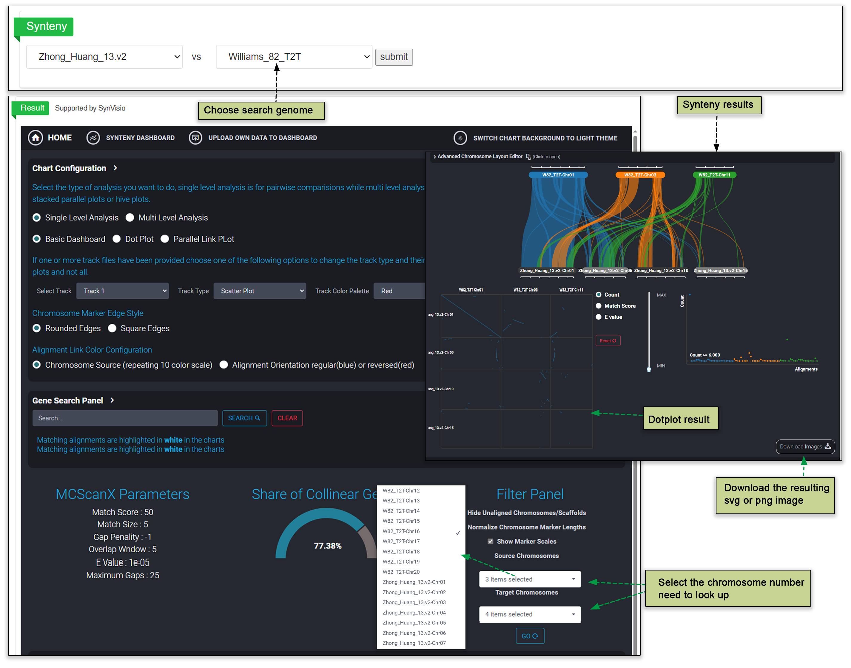
Fig. 22. Synteny visualization using SynVisio.

8.2   Genome synteny

Understanding the direct relationships between genomes is pivotal in genomics research. A collinearity map is constructed to visually represent these results. This map enables researchers to easily discern areas of genetic conservation and divergence across different genomes. By illustrating the linear arrangement of genes, the collinearity map facilitates a deeper understanding of genomic architecture and difference. The genome synteny submodule compares the variation between two genomes at the chromosomal level via a user-friendly interface. Inversion, translocations and duplications can be readily spotted, allowing for precise examination of genomic regions of interest and providing researchers with actionable data on specific genetic variations.

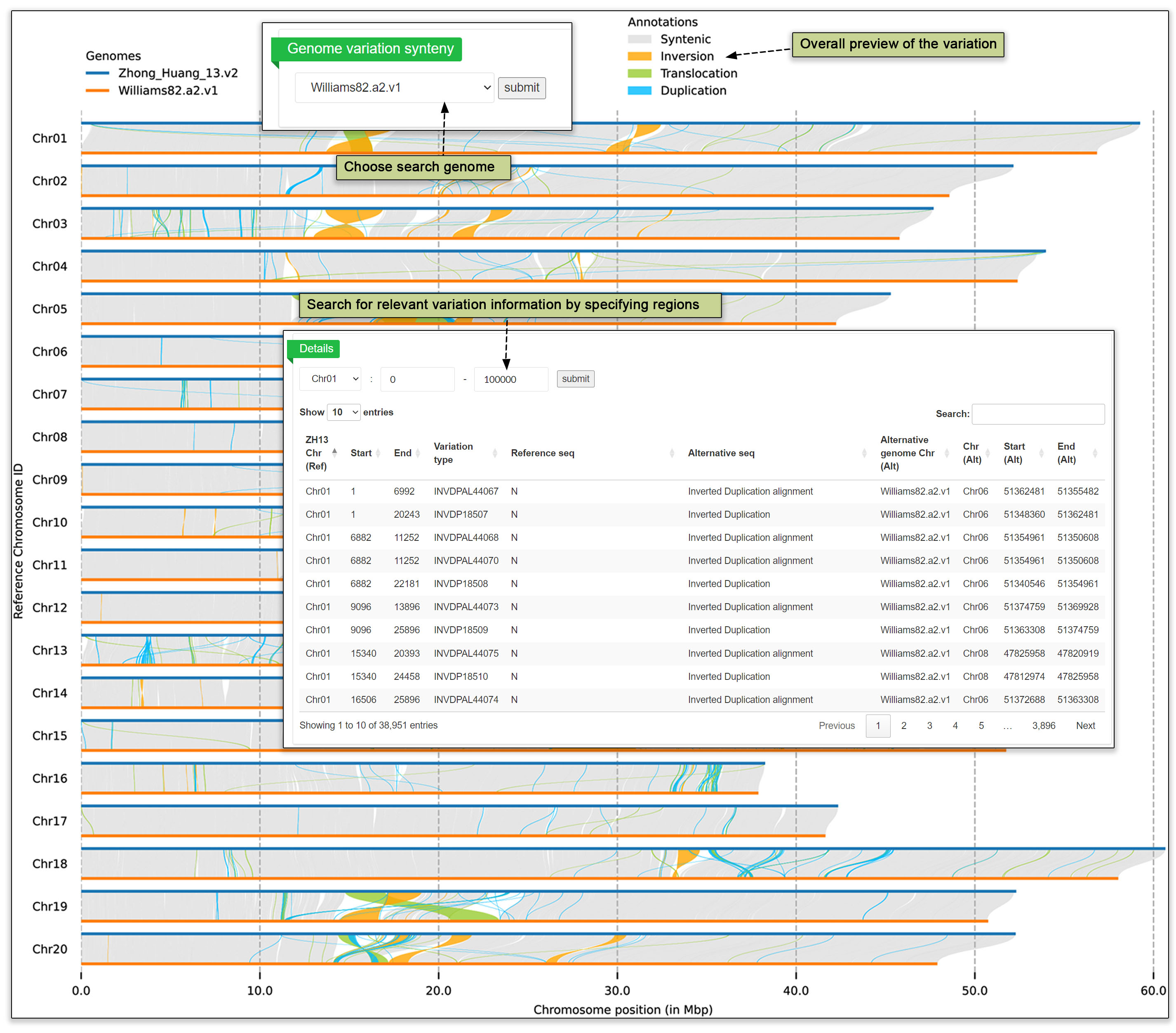
Fig. 23. Visualization of genome synteny in pairwise comparisons.

9.      Toolkits

Several tools are boxed together under the toolkits drop-down menu. These tools allow users to interact with the data contained within SoyOD in different ways, and include the Jbrowse genome browser, BLAST search tool, a way to convert between different versions of the soybean genome, a sequence extraction tool, a heatmap generator, a diversity viewer by chromosome regions, and a haplotype and diversity.

9.1   JBrowse

A genome browser is launched by choosing the JBrowse tool. The Zhonghuang 13 v2 genome is provided as the reference genome. Gene annotation, transcription, variation information can also be viewed.

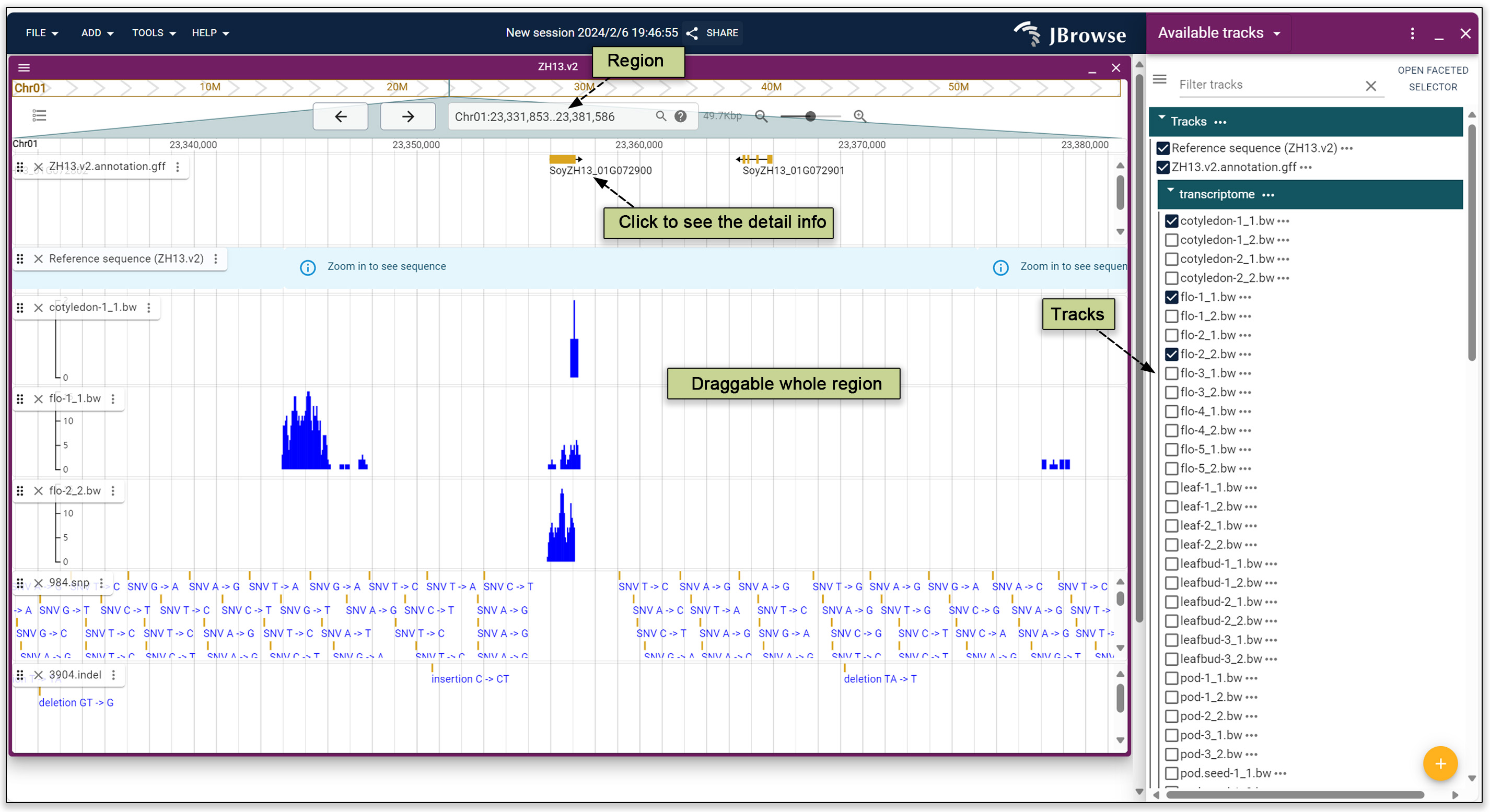
Fig. 24. JBrowse tool.

9.2   BLAST

The genome, coding sequences (CDS), and protein sequences predicted from the 52 sequenced accessions are provided for searches using BLAST. Our platform is designed to comprehensively accommodate research needs. A used can input multiple query sequences simultaneously, enabling efficient and wide-ranging analyses. Additionally, SoyOD supports uploading of sequences, giving a user the flexibility to examine custom data sets alongside our extensive database. To ensure that searches yield the most relevant results, advanced parameters are available for customization. These options allow the user to refine queries based on specific requirements. The combination of versatile input options and sophisticated customization makes our BLAST tool a robust solution for sequence comparisons.

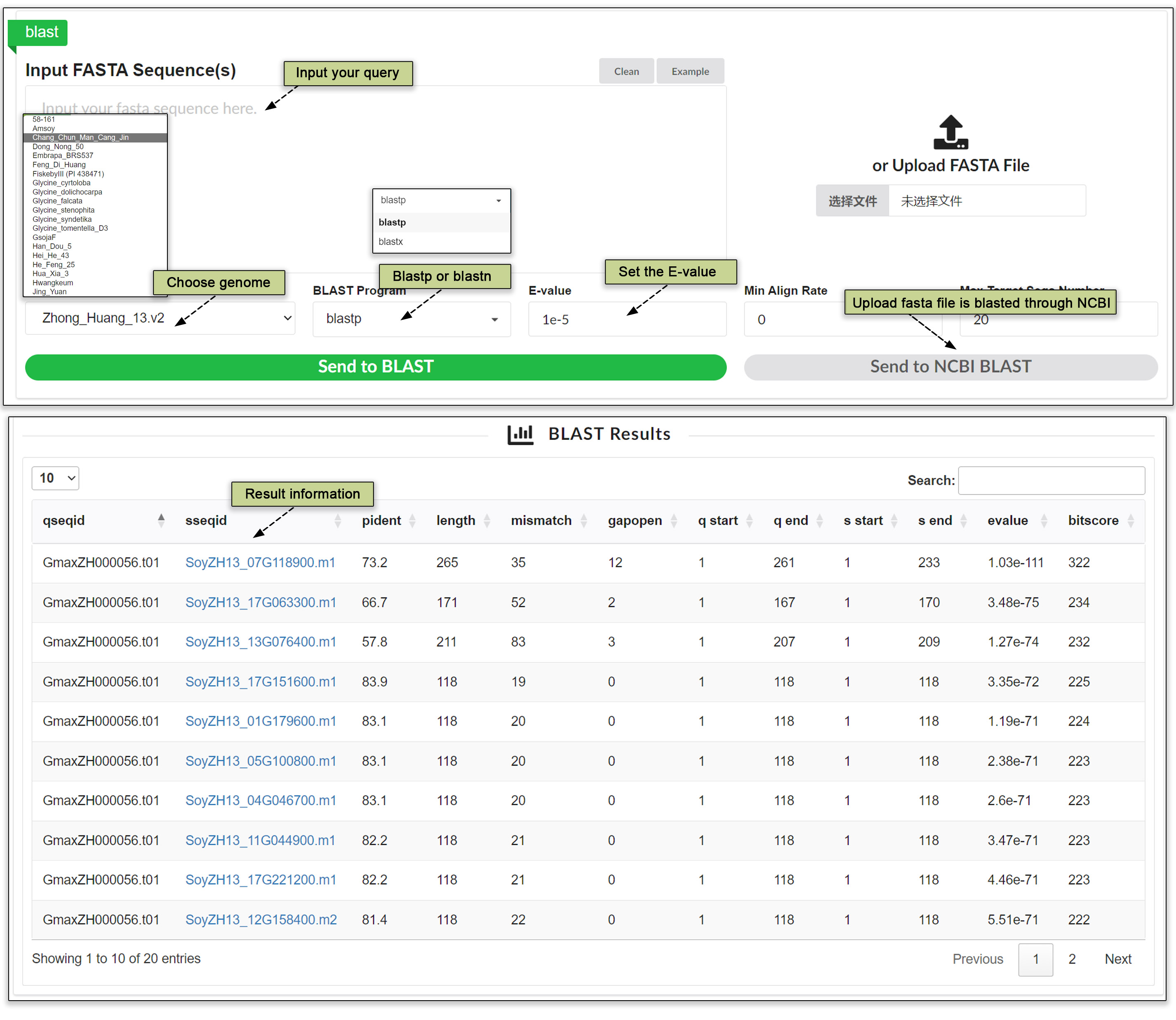
Fig. 25. BLAST search tool.

9.3   Soy-Version convert

The soybean genome version converter facilitates genomic position transformations between the different genome versions. This capability is essential for researchers engaged in comparative genomics, enabling the alignment of genetic data across different soybean genome versions for more effective analysis and interpretation. Our tool offers two distinct conversion models to cater to varied research needs: the gene ID convert model and the genome region coordinate convert model. The gene ID convert model allows researchers to translate gene identifiers from the different genome versions, ensuring consistency in gene identification across studies. On the other hand, the genome region coordinate convert model adjusts genomic coordinates to correspond accurately between different versions, which is crucial for precise genomic mapping and comparison. Both the gene ID and region models are fully supported, providing a comprehensive solution for researchers looking to navigate the complexities of the soybean genome.

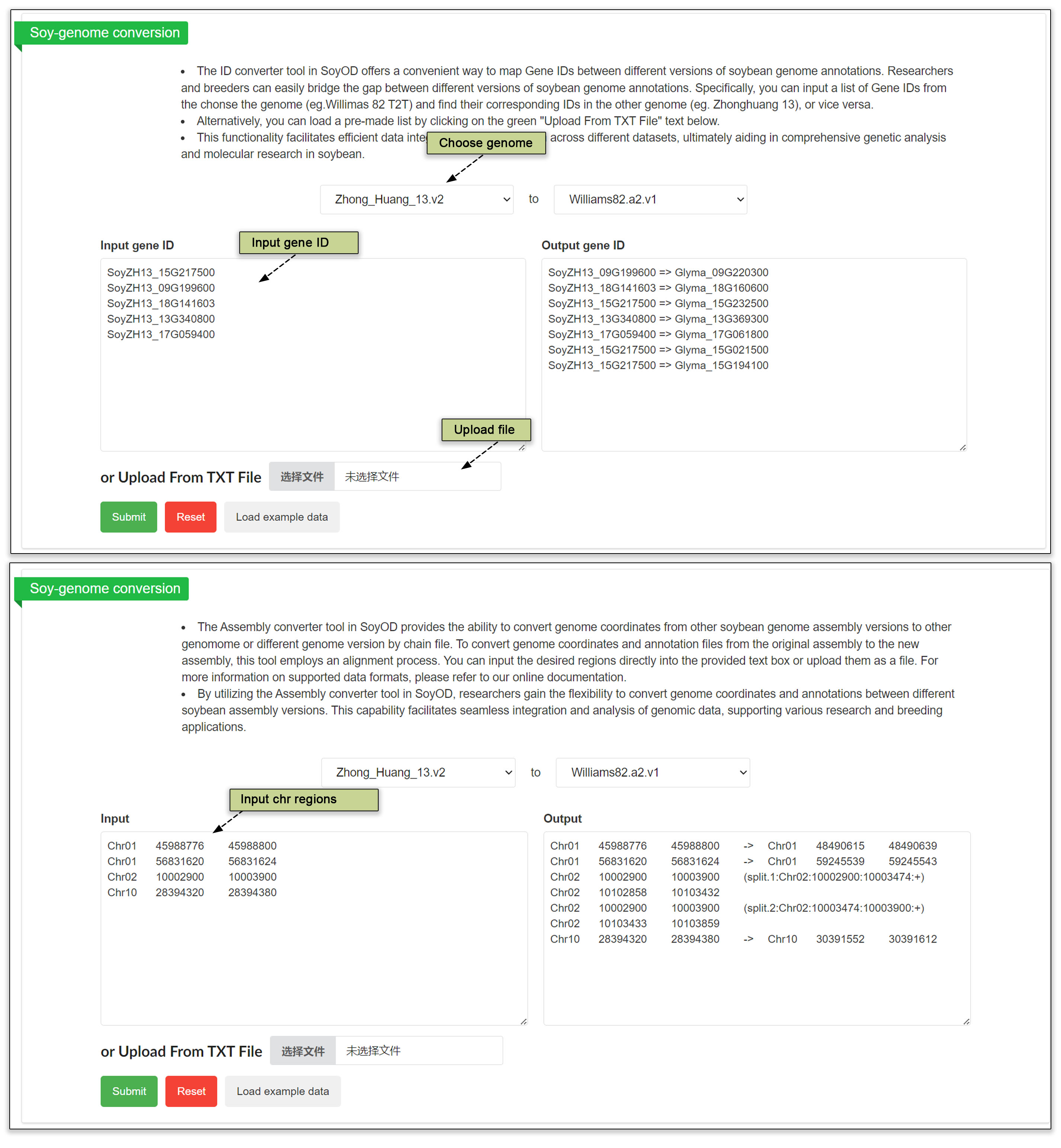
Fig. 26. Soybean genome converter.

9.4   Seq extraction

Sequence extraction is a pivotal tool designed for researchers and scientists engaged in the field of soybean genomics, offering the capability to rapidly access a wide array of genetic sequences across 52 soybean genomes. This tool significantly streamlines the process of obtaining crucial data, such as genomic regions, genes, mRNA, coding sequences (CDS), and proteins, empowering users to conduct thorough and varied analyses. Using Seq extraction is straightforward and efficient: start by selecting your reference genome from the extensive library. Then, specify the type of sequence you wish to extract, whether for a singular query regarding a specific gene or a comprehensive list targeting multiple genomic features. Our user-friendly platform supports both individual and batch queries, ensuring that your research progresses smoothly and swiftly.

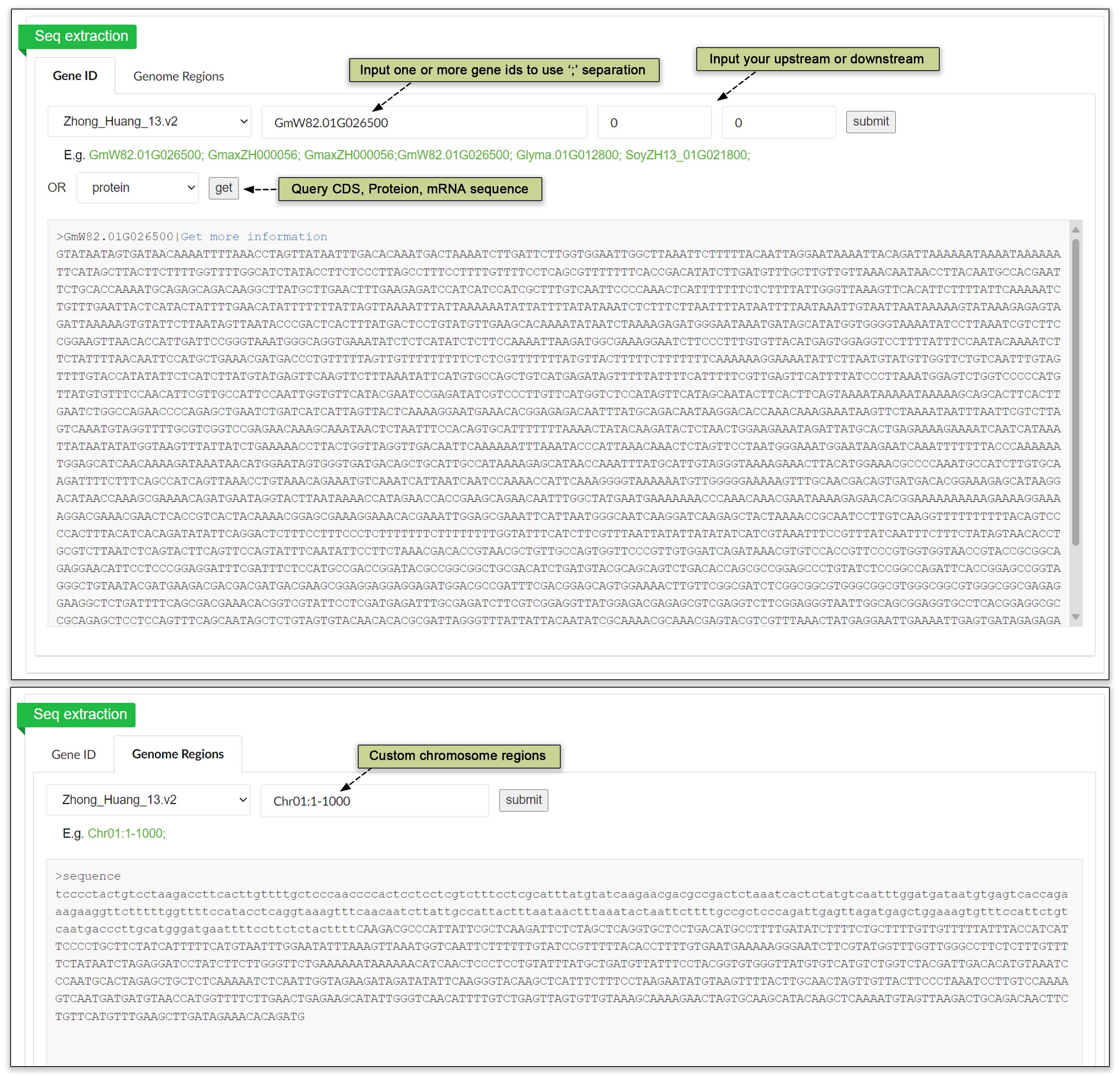
Fig. 27 Sequence extraction using gene IDs or regions.

9.5   Heatmap

Heatmaps are a powerful way to visualize transcriptomic data, enabling researchers to easily identify patterns, variations, and expressional changes within datasets. The heatmap tool in SoyOD offers extensive customization options to tailor the matrix content to specific research needs. Whether a user is analyzing differential gene expression under various conditions or comparing transcriptome profiles across multiple samples, adjusting the matrix content ensures a heatmap that directly addresses the investigative focus. Furthermore, the ability to edit the color scheme and interval settings of the heatmap enhances its utility.

Fig. 28. Custom heatmaps.

9.6   Diversity

We conducted a selective clearance analysis using high-depth sequencing data (984) and all varieties data (3904). Four different analysis methods, including XP-CLR, Fst, Pi ratio, and Tajima’s D, were employed for the whole genome selective test. Users have the flexibility to identify tracks and regions according to their preferences, with a threshold of the top 5% represented by a dashed line. This allows for a more personalized approach to track and analyze genomic regions of interest. Figures presenting the results of the selective test are available for download, facilitating a visual understanding of the data. Furthermore, users can easily observe the selection of genes by accessing gene information through the JBrowse interface. This integration between analysis methods and user-friendly interfaces enhances the accessibility and usability of the data for researchers.

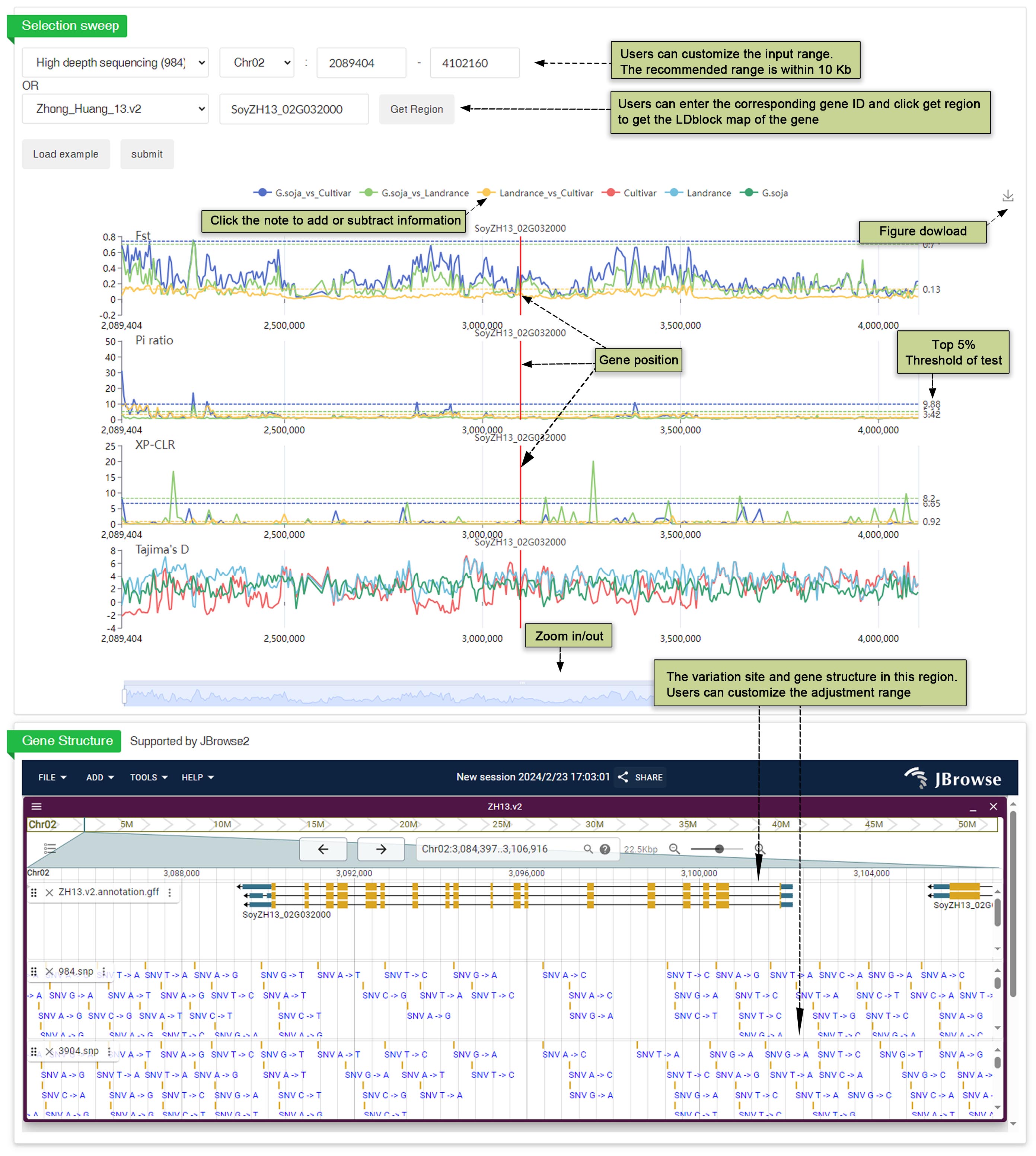
Fig. 29 Diversity search

9.7   Haplotype

This part draws the LD block if the variation is involved in. The R2 value can be set as a threshold for drawing the LD heat map and displaying variations in the table. By setting R2 as a threshold, users can visualize the linkage disequilibrium (LD) pattern more effectively. Additionally, other variations involved in the same LD block can be easily accessed directly from this interface. This streamlined approach allows users to navigate through related variations efficiently. Moreover, users have the option to download the LD heat map for further analysis or reference. Providing the ability to download the LD heat map enhances the usability of the tool and allows researchers to incorporate the data into their own analyses seamlessly. Users have the flexibility to identify tracks and regions according to their preferences. Figures presenting the results of the selective test are available for download, facilitating a visual understanding of the data. Additionally, users can easily observe the selection of genes by accessing gene information through the JBrowse interface.

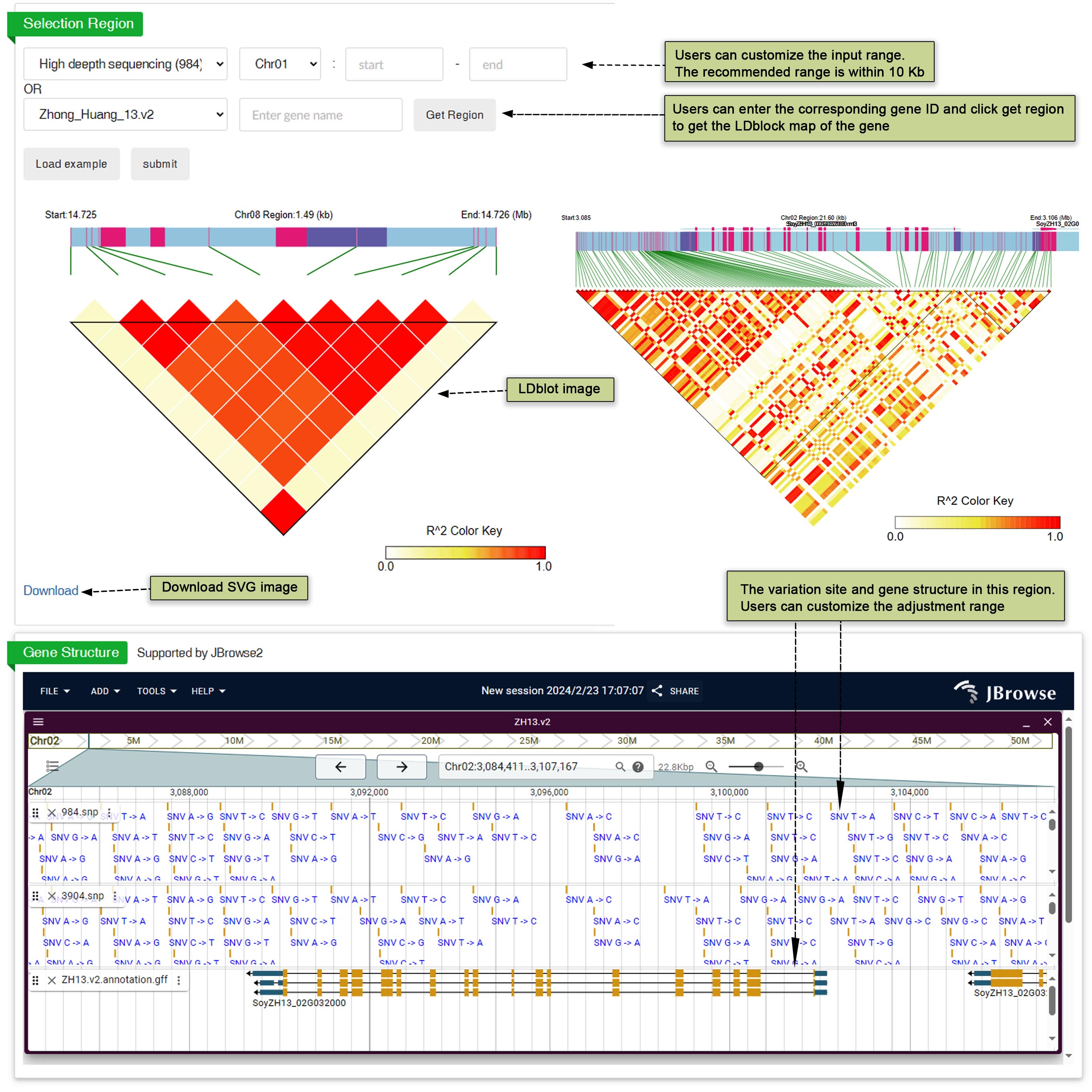
Fig. 30 LD block

10. Download

The download module provides a direct way to download the various information contained within SoyOD and can be accessed through a sortable and searchable table. Genome sequences can be downloaded as GFF or FASTA files, other sequences files related to this genome can be downloaded, including the deduced coding, non-coding, and protein sequences, and a link to the original publication is included. The original publications are listed for the transcriptome, population, variome, and phenome datasets. Text files for transcription factors and transposons (TF/TE) and pathway analysis (GO/KEGG), are also available for downloading.

11. Contact

11.1   Expect and update

SoyOD is dedicated to providing a comprehensive repository of knowledge and a suite of analysis applications tailored for one-stop soybean multi-omics research. Our platform covers a wide range of omics data, alongside powerful tools designed for in-depth data analysis, insightful visualization, and seamless data integration. This combination empowers researchers to conduct holistic and efficient studies on soybean biology.

We are committed to keeping SoyOD at the forefront of soybean research through regular updates. These enhancements will include incorporating the latest scientific discoveries, refining existing tools for greater accuracy and ease of use, and introducing innovative features in response to the needs and feedback of our user community. Our goal is to ensure that SoyOD remains not only robust and reliable, but also increasingly convenient and user-friendly. Users gain access to a wealth of resources that streamline the research process, deepen insights into the complex mechanisms underlying soybean biology, and potentially pave the way for novel discoveries in the field. We invite researchers, educators, students, and anyone interested in soybean science to explore what SoyOD has to offer and to join us in enriching this platform with your insights, research findings, and feedback.

Together, let's explore this wealth of knowledge and the untapped potential of this vital crop through the integrated soybean molecular data provided by SoyOD.

11.2 Funding 

This work was supported by the Ministry of Science and Technology of China (2021YFF1000402); Zhejiang Province key research and development project (2021C02057, 2021C02053). National Natural Science Foundation of China (32270709, 32261133526, 32300532).

11.3   Contact us

We value your insights and are eager to address any questions or comments you may have. You can find our contact details here. We look forward to hearing from you and engaging in meaningful conversations.

State Key Laboratory of Plant Environmental Resilience, College of Life Sciences, Zhejiang University, Hangzhou, Zhejiang 310058, China

Ø  Telephone: +86-(0)571-88206146

Ø  Fax: +86-(0)571-88206146

Ø  E-mail: Huixia Shou (huixia@zju.edu.cn); Jie Li (jieli3@zju.edu.cn)

Ø  E-mail: Ming Chen (mchen@zju.edu.cn); Qingyang Ni (qingyangni@zju.edu.cn)

12. Reference

1. Zhang, C., Xie, L., Yu, H., et al. (2023). The T2T genome assembly of soybean cultivar ZH13 and its epigenetic landscapes. Molecular plant, 16(11), 1715–1718.

2. Wang, L., Zhang, M., Li, M., Jiang, X., Jiao, W., & Song, Q. (2023). A telomere-to-telomere gap-free assembly of soybean genome. Molecular Plant, 16(11), 1711–1714.

3. Liu, N., Niu, Y., Zhang, G., et al. (2022). Genome sequencing and population resequencing provide insights into the genetic basis of domestication and diversity of vegetable soybean. Horticulture research, 9, uhab052.

4. Zhuang, Y., Wang, X., Li, X., et al. (2022). Phylogenomics of the genus Glycine sheds light on polyploid evolution and life-strategy transition. Nature plants, 8(3), 233–244.

5. Chu, J. S., Peng, B., Tang, K., et al. (2021). Eight soybean reference genome resources from varying latitudes and agronomic traits. Scientific data, 8(1), 164.

6. Sun, S., Yi, C., Ma, J., et al. (2020). Analysis of Spatio-Temporal Transcriptome Profiles of Soybean (Glycine max) Tissues during Early Seed Development. International journal of molecular sciences, 21(20), 7603.

7. Liu, Y., Du, H., Li, P., et al. (2020). Pan-Genome of Wild and Cultivated Soybeans. Cell, 182(1), 162–176.e13.

8. Wang, S., Liu, S., Wang, J., et al. (2020). Simultaneous changes in seed size, oil content and protein content driven by selection of SWEET homologues during soybean domestication. National science review, 7(11), 1776–1786.

9. Wang, S., Yokosho, K., Guo, R., et al. (2019). The Soybean Sugar Transporter GmSWEET15 Mediates Sucrose Export from Endosperm to Early Embryo. Plant physiology, 180(4), 2133–2141.

10. Valliyodan, B., Cannon, S. B., Bayer, P. E., et al. (2019). Construction and comparison of three reference-quality genome assemblies for soybean. The Plant journal: for cell and molecular biology, 100(5), 1066–1082.

11. Xie, M., Chung, C. Y., Li, M. W., et al. (2019). A reference-grade wild soybean genome. Nature communications, 10(1), 1216.

12. Shen, Y., Du, H., Liu, Y., et al. (2019). Update soybean Zhonghuang 13 genome to a golden reference. Science China. Life sciences, 62(9), 1257–1260.

13. Pelletier, J. M., Kwong, R. W., Park, S., et al. (2017). LEC1 sequentially regulates the transcription of genes involved in diverse developmental processes during seed development. Proceedings of the National Academy of Sciences of the United States of America, 114(32), E6710–E6719.

14. Shen, Y., Zhou, Z., Wang, Z., et al. (2014). Global dissection of alternative splicing in paleopolyploid soybean. The Plant cell, 26(3), 996-1008.

15. Schmutz, J., Cannon, S. B., Schlueter, J., et al. (2010). Genome sequence of the palaeopolyploid soybean. Nature, 463(7278), 178–183.

16. Grant, D., Nelson, R. T., Cannon, S. B., et al. (2010). SoyBase, the USDA-ARS soybean genetics and genomics database. Nucleic acids research, 38(Database issue), D843–D846.